First steps with PyAnsys using an end-to-end example
Aileen Lützke
20.12.2024
Tech Article 24/18 | PyAnsys: Automation Made Easy
Is your desk also full of simulation tasks? Using a small workflow, we will show you how you can automate simulations with PyAnsys and make them run error-free and standardized. This allows you to save valuable time which can then be used to explore new fields and test out ideas.

© Adobe Stock
PyAnsys: A Bridge between Ansys and Python
Have you ever thought of simply running simulation workflows in Ansys in the background, completely automatically, error-free and standardized? Have you already heard of PyAnsys and have an affinity for programming, but haven't had the time to read up on it yet? In this article, we would like to show you how easy it is to get started with PyAnsys. With PyAnsys, you can automatically adapt and modify geometries, carry out simulations and automate the post-processing of results in Ansys to save time and effort.

PyAnsys – A bridge between the power of Ansys simulation tools and the Python ecosystem | © CADFEM Germany GmbH
Here’s what’s new about PyAnsys: PyAnsys offers a broad range of applications for the automation and customization of workflows that goes beyond individual Ansys products and makes the entire Ansys ecosystem accessible via Python. In-product scripting was and is limited to the specific product in which it is implemented. PyAnsys, on the other hand, offers seamless integration and collaboration between various Ansys products and Python libraries, much like a bridge. Of course, PyAnsys also requires a certain amount of training, but Ansys provides extensive resources such as documentation, tutorials and community forums to help you learn and grow.
Using a simple workflow, including geometry preparation with PyAnsys Geometry and simulation setup with PyMechanical, we would like to show how processes can be standardized across projects and teams. In addition, you can use custom script libraries to extend the automation possibilities beyond Ansys and take advantage of the compatibility of PyAnsys with other Python libraries and tools. Embedded in a web application, this results in an easy-to-use tool even for inexperienced users. Automation increases efficiency, reduces errors and, above all, frees up time to tackle higher-value tasks.
A collection of Python libraries in the Ansys environment
Ansys offers a wide range of modules. A very good overview can be found under the following link: PyAnsys. For each module, there are comprehensive user manuals, API references and examples that make learning and using the respective Ansys tools simple. As part of the PyAnsys ecosystem, these modules are regularly updated to support new versions and updates of the corresponding Ansys software.
Ansys categorizes the PyAnsys modules into three main groups:
-
Simulation Libraries
-
Utility Libraries
-
Postprocessing Libraries
Simulation libraries enable automated simulations such as PyMAPDL (Ansys Mechanical), PyAEDT (Ansys Electronics) and PyFluent (Ansys Fluent). Utility libraries offer general functionalities such as the processing of geometries (PyAnsys Geometry) or the creation of meshes (PyPrimeMesh). The PyDynamicReporting module enables the creation of diagrams, animations or images from the simulation results in order to derive valuable insights. The PyDPF modules focus on the extraction and post-processing of simulation results for evaluations, reporting or further use in downstream analyses.
Thanks to the neutral interfaces, generated data can be reused in other Python modules and allowing complex, multidisciplinary problems to be solved.
The Python world generally offers a large number of helpful libraries:
- Numpy is a numerical library for easier processing of n-dimensional data.
- Scipy is based on NumPy and supports calculations such as numerical integration, optimization, interpolation, signal processing and much more.
- Matplotlib is a data visualization library in Python that can be used to create charts, histograms, bar charts, scatter plots, etc. with just a few lines of code
- PyVista supports the visualization of data/models in 3D.
- Pandas – Reading, writing and processing table data (Excel)

Overview PyAnsys categories | © CADFEM Germany GmbH
Every beginning with PyAnsys is difficult - or is it?
The fastest way to learn something is to do it yourself, preferably in a familiar environment. PyAnsys can be written and executed in any integrated development environment (IDE) that can run Python code. To simplify debugging, we use JupyterLab, an open source tool that can be used to run the Python code interactively. The Ansys installation can be used as a basis to create a virtual Python environment, without the need for a new Python installation. Ansys provides an Ansys Python Manager in the Ansys Developer Portal for this purpose (Ansys Python Manager).
The Ansys Python Manager guides you through the creation of the virtual Python environment and the installation of the PyAnsys packages in just a few steps. When you install the PyAnsys metapackage, you install the full scope of PyAnsys libraries. Please install the correct Python version. It is recommended to install the latest Python version in the current Ansys version.
After successful installation, you have 2 options via the Ansys Python Manager. With one click, you can start the JupyterLab, in which you can develop your first PyAnsys example. If you have installed several versions, make sure you select the correct Python environment. To quickly execute and test short lines of code, you can also start a console via the Manager. Let's now get started and take a look at an example from geometry preparation to simulation.

The Ansys Python Manager - Simplified management of the Python environment | © CADFEM Germany GmbH
From geometry processing to the results with PyAnsys
If you have your Python environment ready to go, we can get started together. In the following sections, we will use PyAnsys Geometry to import a geometry, prepare it and save it for further processing in Mechanical. With PyMechanical, we set the boundary conditions, analysis settings, calculate the simulation model and save the results as a 3D result. In our case, this is a simple bracket that is deformed by a small load.
But what can actually be done with PyAnsys Geometry? PyAnsys Geometry is a Python client library for the Ansys Geometry service and can therefore be used via Docker, locally or remotely. In most cases, the models have been created in CAD systems. These can be imported, topologically analyzed and post-processed for the simulation, such as editing or creating named selections for targeted selections for further use in the calculation processes. You can even use the Sketch and Shape functions to create simple geometries.
PyMechanical is a module for the modeling, simulation and analysis of mechanical systems based on an existing geometry. Just like interactively in Mechanical and beyond, you have access to elements, material properties, contacts, loads and boundary conditions, and can perform static and dynamic, linear and non-linear analyses. PyMechanical thus bridges the gap between geometry creation and results visualization. As with all PyAnsys modules, it is compatible with other Python libraries, enabling the creation of efficient, reliable and interoperable workflows.

Tip
Automation and Digitalization with PyAnsys
Streamline workflows and gain deeper insights into simulations.
PyAnsys Geometry – the initial step
We use Ansys Discovery to process the geometry. Among other things, PyAnsys Geometry is able to connect to a running session of Discovery or SpaceClaim or create a new session where it can use the functionalities:
from ansys.geometry.core import launch_modeler_with_discovery
modeler = launch_modeler_with_discovery()
To open the geometry, the paths must be created automatically. In our case, the geometry is located in the same directory as the Python script:
import os
fd = os.getcwd()
des_fp = os.path.join(fd,"data","bracket_with_ns.scdoc")
design = modeler.open_file(des_fp)
Our geometry has many small roundings and chamfers. To speed up meshing and simulation, we select and remove roundings with a radius of less than 0.2 mm and chamfers with a length of less than 0.5 mm. Discovery already has ready-made functions for this, which can be used very smartly.
For the roundings, it looks like this: Select using the Power Select method and remove using the Fill method.
selection = PowerSelection.Faces.ByRoundRadius(MM(0.2), PowerSelectOptions(False, Selection.Create(GetRootPart().Bodies[1])), SearchCriteria.SizeComparison.SmallerOrEqual,
SearchCriteria.RoundType.All)
secondarySelection = Selection.Empty()
options = FillOptions()
result = Fill.Execute(selection, secondarySelection, options, FillMode.ThreeD, None)
For chamfers, the Power Select() command changes slightly, but in principle is similar:
selection = PowerSelection.Faces.ByChamferLength(MM(0.5),PowerSelectOptions(False, Selection.Create(GetRootPart().Bodies[1])),SearchCriteria.SizeComparison.SmallerOrEqual)

Geometry with chamfers and roundings - Prepared with PyAnsys Geometry | © CADFEM Germany GmbH
Work in a structured way. For the second use at the latest, it is worth writing a sub-function. Here is an example of our defeaturing task: If you pack the lines of code into a separate function, you have the option of setting default values and also adjusting these by calling them:
def remove_fillets_chamfers(fillet_radius=0.2,chamfer_length = 0.5):
#Fillets
selection = PowerSelection.Faces.ByRoundRadius(MM(fillet_radius),
PowerSelectOptions(False, Selection.Create(GetRootPart().Bodies[1])),
SearchCriteria.SizeComparison.SmallerOrEqual,
SearchCriteria.RoundType.All)
secondarySelection = Selection.Empty()
options = FillOptions()
result = Fill.Execute(selection, secondarySelection, options, FillMode.ThreeD, None)
# Chamfers
selection =
PowerSelection.Faces.ByChamferLength(MM(chamfer_length),PowerSelectOptions(False,
Selection.Create(GetRootPart().Bodies[1])),SearchCriteria.SizeComparison.SmallerOrEqual)
secondarySelection = Selection.Empty()
options = FillOptions()
result = Fill.Execute(selection, secondarySelection, options, FillMode.ThreeD, None)
# Function Call
remove_filltes_chamfers()
If these are saved in a separate library file, they can be called up as follows:
import os
fd = os.getcwd()
fp = os.path.join(fd,"scdm_functions.py")
des_fp = os.path.join(fd,"data","bracket_with_ns.scdoc")
design = modeler.open_file(des_fp)
result,design = modeler.run_discovery_script_file(file_path=fp,script_args={},import_design=True)
path_clean_geom = os.path.join(fd,”cleaned_geom_bracket.scdoxc”)
PyMechanical: From geometry to simulation model
We can now use the geometry we've prepared for the model setup in PyMechanical. In our case, attributes are already defined on the surfaces in the CAD model in the form of named selections in order to achieve an efficient model setup.
from ansys.mechanical.core import launch_mechanical
mechanical = launch_mechanical(batch=True)
def attach_geometry(path_clean_geom):
geometry_import_group = Model.GeometryImportGroup
geometry_import = geometry_import_group.AddGeometryImport()
geometry_import_format = (
Ansys.Mechanical.DataModel.Enums.GeometryImportPreference.Format.Automatic
)
geometry_import_preferences = Ansys.ACT.Mechanical.Utilities.GeometryImportPreferences()
geometry_import_preferences.ProcessNamedSelections = True
geometry_import.Import(part_file_path, geometry_import_format, geometry_import_preferences)
return "success"
If you are not yet familiar with mechanical scripting, open Mechanical interactive and simply record the manual steps (Ansys Mechanical à Tab Automation à Button Scripting à Start Recording). These can then be applied 1:1.
The basis for many model setup methods is the ExtAPI.DataModel.Project.Model object. The sub-methods for creating boundary conditions, contacts and meshing can be found here. The structure is similar to the object tree in Mechanical, making it easy, also with the help function, to find the correct method or object.
contact_container = ExtAPI.DataModel.Project.Model.Connections
mesh_container = ExtAPI.DataModel.Project.Model.Mesh
The simulation model can now be built up successively on the basis of geometry selection or, in our case, on named selections. The name of the named selection (e.g. faces) can be accessed as follows:
sel_info = DataModel.GetObjectsByName(“Name_Named_Selection”).Location
The sel_info object can then be used for further functions, i.e. for creating boundary conditions or contact conditions, similar to what you are used to interactively:
# create new contact
sel_info_contact = DataModel.GetObjectsByName(“NS_contact”).Location
sel_info_target = DataModel.GetObjectsByName(“NS_target”).Location
contact_region = contact_container.AddContactRegion()
contact_region.SourceLocation =sel_info_contact #Kontaktseite
contact_region.TargetLocation = sel_info_target # Targetseite
contact_region.ContactType = ContactType.Frictional
#create mesh
element_size = 3 # in mm
element_size_quantity = Quantity(element_size,'mm')
mesh_container = ExtAPI.DataModel.Project.Model.Mesh
mesh_container.ElementSize = element_size_quantity
mesh_container.UseAdaptiveSizing = False
mesh_container.GenerateMesh()
As in the Mechanical tree, boundary conditions are also located below the analysis object:
#Set Boundary Conditions
analysis = ExtAPI.DataModel.Project.Model.Analyses[0]
sel_info_support = DataModel.GetObjectsByName(“NS_support”).Location
remote_displacement = analysis.AddRemoteDisplacement()
remote_displacement.Location = sel_info_support
remote_displacement.XComponent.Output.DiscreteValues=[Quantity(0, "mm")]
remote_displacement.YComponent.Output.DiscreteValues=[Quantity(0, "mm")]
remote_displacement.ZComponent.Output.DiscreteValues=[Quantity(0, "mm")]
remote_displacement.RotationX.Output.DiscreteValues=[Quantity(0, "grad")]
remote_displacement.RotationY.Output.DiscreteValues=[Quantity(0, "grad")]
remote_displacement.RotationZ.Output.DiscreteValues=[Quantity(0, "grad")]
sel_info_bc = DataModel.GetObjectsByName(“NS_bc”).Location
displacement = analysis.AddDisplacement()
displacement.Location = sel_info_bc
displacement.XComponent.Output.DiscreteValues=[Quantity(0, "mm")]
displacement.YComponent.Output.DiscreteValues=[Quantity(-0.1, "mm")]
displacement.ZComponent.Output.DiscreteValues=[Quantity(0, "mm")]
The properties can be adjusted for all these methods, just as in interactive work. When programming, pay particular attention to units and alignment in the coordinate system. These two factors are major sources of error in automation.

Automating model setup with PyAnsys | © CADFEM Germany GmbH
PyMechanical: Results and evaluation
To evaluate the results after the simulation, we add post-processing objects for the total deformation and the Von Mises stresses to our model. Here too, the same structure applies as you are used to in Mechanical. The results are inserted below the Solution object, a child object of the Analysis object.
# Set Results
analysis = ExtAPI.DataModel.Project.Model.Analyses[0]
analysis.Solution.AddTotalDeformation()
analysis.Solution.AddEquivalentStress()
The selection objects can also be used here for individual bodies:
sel_info_def = DataModel.GetObjectsByName(“NS_tot_def”).Location
total_deformation = analysis.Solution.AddTotalDeformation()
total_deformation.Location = sel_info
And last but not least, please don't forget to save it!
ExtAPI.DataModel.Project.Save(file_path)
In the best case scenario, you will have written the individual steps of the functions when reprogramming and can now build the model clearly in one step at the end:
mechanical.run_python_script(f"attach_geometry(r'{fp}')")
mechanical.run_python_script("an=Model.AddStaticStructuralAnalysis()")
mechanical.run_python_script("create_contact('NS_contact','NS_target')")
element_size = 3 # in mm
mechanical.run_python_script(f"set_mesh({element_size})")
mechanical.run_python_script("set_bc('NS_support','NS_bc')")
mechanical.run_python_script("set_result()")
mechanical.run_python_script("an.Solve()")
If you are using your automation for end-to-end workflows, images and the report are of course still missing. Retrieve the corresponding result object from the tree and create images. Ansys also offers the option of different camera settings for this. If the views cannot be clearly defined as a result of the models changing considerably, it may make more sense to create a 3D file. Ansys exports avz files, for example, which can then be viewed later via external viewers or integrated into an HTML report.
sol = analysis.Solution
results = sol.GetChildren(DataModelObjectCategory.Result,True)
export_setting = Ansys.Mechanical.Graphics.GraphicsImageExportSettings()
res[0].Activate()
Graphics.Camera.SetFit()
#Export Image
f_name = "{0}_{1}.png".format(res.Name,res.ObjectId)
f_path = os.path.join(fd,f_name)
Graphics.ExportImage(f_path,GraphicsImageExportFormat.PNG,export_setting)
#Export 3D Image
f_name = "{0}_{1}.avz".format(res.Name,res.ObjectId)
f_path = os.path.join(fd,f_name)
Graphics.Export3D(f_path,Graphics3DExportFormat.AVZ,export_setting)

Simulation results - obtained completely automatically | © CADFEM Germany GmbH
PyDynamicReporting: How does it work with reporting?
Do you like writing reports? With PyDynamicReporting, you can now automatically create reports based on predefined templates, reducing manual effort and ensuring a consistent layout across multiple reports. Previously generated images and 3D images can be integrated quickly and easily. The report can be exported to various file formats, such as PDF, HTML and Microsoft Office Suite documents(beta). You will see that writing reports (or having them written) is fun again.

Model setup and reporting – time-consuming and expensive | © CADFEM Germany GmbH
A few tips to conclude with: comment on your code, because after a while, even as a developer, you forget what your thoughts were at the time. This is also helpful for your colleagues, who may have to familiarize themselves with it later. Write a log file for the end users so that errors can be found and rectified more quickly. And “Nobody is perfect”. When setting up automation, keep in mind that users can also make mistakes when entering data. You should therefore try to anticipate and catch these at an early stage using value ranges, input types and units.
Of course, this was only a brief insight using a simple example. However, I hope that the hurdle of taking the time to familiarize yourself with PyAnsys has been overcome. Please also take a look at our Python-Training, which continue from where this article leaves off, making it even easier to get started. If you can see the benefits of automation, but lack the know-how and time to implement it, please contact us and we will find a solution together.
Training on the topic
-
Python Primer for Ansys

In this training, you will learn the basics of Python programming for using PyAnsys and automating your Ansys simulations.
-
Using Python to Automate Tasks within Ansys Maxwell

In this training, you will learn to use the IronPython interface as well as PyAEDT libraries and API to automate workflows in Ansys Maxwell.
-
Automation within Ansys Mechanical Using Python

Learn how to write your own scripts: from automatic geometry selection to standardized reports.
-
Automation of Fluent using PyFluent

In this course, you will learn how to control and automate your Ansys Fluent flow simulation using PyFluent.
-
Automation with Ansys Discovery Scripting

In this training course, you will learn to control Ansys Discovery via the script language Python: from geometry to simulation.


Technical Editorial
Dr.-Ing. Marold Moosrainer
Head of Professional Development
+49 (0)8092 7005-45
mmoosrainer@cadfem.de


