How do I use the NVH Toolkit in Ansys?

In parallel to numerical modal analysis, in which the natural frequencies and modes of a structure are calculated using the mass, damping and stiffness matrix, experimental modal analysis (EMA) is used to determine the natural frequency, the associated modal damping, and the natural modes of vibration on physical components. Instead of solving an eigenvalue problem, the structure is excited to vibrate, and the response is measured at discrete points. This allows transfer functions to be formed between response and excitation, from which the modal parameters and the vibration modes of a component can be determined using special curve fitting.

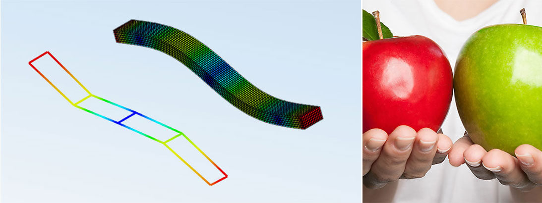
But how can natural modes and frequencies from simulation and testing be compared with each other? It is easy to determine the difference between a measured natural frequency and the corresponding simulated natural frequency. The result is a scalar numerical value. But how do you determine which vibration mode from measurement and calculation belong together? Without a way to visualize these modes side by side, this is hardly possible. The NVH Toolkit has been available in Ansys Mechanical since 2022 R1! It can be activated in the Add-Ons tab. The so-called MAC Calculator is then added to the results in a modal analysis. But how do we get our measurement data loaded there?

Activation of the NVH Toolkit in Ansys Mechanical and insertion of the MAC Calculator in a modal analysis | © CADFEM Germany GmbH

Import test data in Universal File Format (UNV)

There are many ways to carry out an EMA - from pulse hammers and accelerometers to excitation via shakers or loudspeakers and measuring the response with 3D laser vibrometers. The manufacturers of measuring equipment often use proprietary file formats that cannot be read without the associated software. This is why the Laboratory for Structural Dynamics at the University of Cincinnati defined the Universal File Format (*.unv or *.uff). This standard describes a pure text file and can be exported from almost any measurement software. The file contains text blocks that are referred to as formats and, depending on their content, adhere to a predefined structure (measurement point coordinates, eigenmodes) [1].

In this article, we look at a simple steel beam for which a measurement is available. This contains a total of ten different measuring points and the first six eigenmodes. In Ansys Mechanical, all we have to do is enter the path to the corresponding measurement file in the details window. The information read from the UNV file is then automatically displayed in the graphics window. We can see the measurement grid used in red so that we can directly recognize the extent to which the orientation matches our simulation model. If necessary, we can also correct the orientation or scaling directly in the MAC Calculator.

Visualization of the measuring grid from the UNV file on the simulation model | © CADFEM Germany GmbH

Visual comparison of the mode shapes

After an update of the results, the view shows a matrix display with coloured cells that represent the simulated modes row by row and those from the UNV file column by column - a comparison of the two worlds. To visualise two modes side by side for comparison, click in the corresponding field of the matrix. The FE result is then displayed in the graphics window on the left and the measured mode on the measuring grid on the right. A side-by-side animation of the paired modes is also possible. This allows us to make an initial subjective assessment of what belongs together. Does this mean that we now have to play "mode memory" and the path to automation is blocked by all the looking?

Simulated 2nd eigenmode (left), measured 3rd eigenmode (right) | © CADFEM Germany GmbH

The Modal Assurance Criterion (MAC)

Let's take another look at this MAC matrix. Behind it is the Modal Assurance Criterion (MAC), which is a correlation criterion for eigenmodes. It provides information on how "related" two mode shapes are to each other. For all indices i and j, the possible mode combinations from FEM and EMA are calculated according to

Does that remind you of anything? Probably the scalar product in geometry to determine the angle between two vectors. Normalization results in values between 0 and 1 for the MAC value, with MAC values close to 1 meaning a high level of agreement between eigenmodes and 0 meaning no agreement at all.

This criterion can therefore also be used to assign mode shapes - so-called mode pairing. Mode pairs are formed based on the highest match. Visual puzzling is no longer necessary, and we have all the trump cards for an automatable workflow in our hands. The Pair Modes option can be activated in the MAC Calculator for this purpose. It is advisable to reduce the MAC limit of 0.9 and, if necessary, the frequency tolerance so that a partner is found for every measured mode. In our case, it is clear to see that all six vibration modes of the measurements can be identified in the simulation, but the order is reversed.

MAC matrix before mode pairing (left) and after (right) | © CADFEM Germany GmbH

Calibration of dynamic simulations with tests

But what should be done if mode pairs are found, but large deviations, e.g. in the frequency, are diagnosed? The MAC provides us with an objective quality criterion for the correspondence of eigenmodes as a numerical value, which also allows automatic mode pairing. An objective function for optimization can be derived from this. The deviation between simulation and test is minimized by varying uncertain simulation parameters (material parameters, physical contact parameters, etc.) with the aim of identifying these. This workflow can be set up with Ansys optiSLang in the Workbench. We will see how this works in practice in the linked CADFEM training!

Model calibration workflow with optiSLang in Workbench (left) and final result with 1.6% (originally 25%) average frequency deviation (right) | © CADFEM Germany GmbH

Cover images: Left: © CADFEM GmbH | Right: © Adobe Stock
Published: May, 2024

References:
[1]: Structural Dynamics Research Laboratory (University Cincinnati) -  Universal File Formats for Modal Analysis Testing (uc.edu) (Stand: April 2024)