MRI despite implant? Simulation protects against heat damage
Dr.-Ing. Jörg Neumeyer
17.07.2025
TechArticle 25/07 | Simulation analyzes risks and optimizes MRI use
Magnetic resonance tomographs are now state of the art for diagnostic purposes in medical technology. However, the electromagnetic fields required for this can have negative effects on the body, organs and, in particular, metallic implants. Simulation can be used to analyze whether and how an MRI examination is possible despite an implant.

Virtual Patient in MRI | © Adobe Stock/CADFEM Germany GmbH
Just look, don’t touch!
Diagnostic imaging procedures in medical technology make a major contribution to the treatment of various diseases and injuries. The particular advantage lies in the fact that the areas of the body being examined can be analyzed without mechanical intervention in the complete cross-section and thus also in deep tissue layers. While imaging procedures based on X-ray radiation can have negative long-term effects due to this very radiation, MRI examinations only have reversible effects during the exposure period. Anyone who has already undergone an MRI can tell you about the loud noise, but we will not go into that today.
The MRI uses both a static magnetic field and a time-varying field for the examination. The static field is used to generate a preferred alignment of the atomic nuclei with a dipole moment via the magnetic moments of the protons. The stronger the field, the clearer the alignment. But the static field also has negative effects. So-called phosphons (small flashes in the eye), magnetic forces on ferromagnetic parts in the body, magnetohydrodynamic effects (relevant for blood pressure) or even Lorentz forces on active implants can result. The strength of the static field influences the necessary excitation frequency in the alternating field.
Perhaps you can imagine the principle as being similar to a toy spinning top. If the spinning top spins quickly, it stands upright. The magnetic moment in the proton spin also rotates faster “and more upright” with large static magnetic fields. According to the so-called Larmor condition, an excitation frequency of approx. 42 MHz is required for hydrogen nuclei per 1 Tesla base field. When using a corresponding high-frequency alternating field, the moment axes are actively tilted in turn and the resulting response to this excitation provides doctors with the information they need to make a diagnosis.
Imaging diagnostics using an MRI | © Adobe Stock
Electromagnetic fields in MRI
The natural “ingredients” of the body consist largely of water and are slightly more or less electrically conductive depending on their composition. From an electromagnetic point of view, it is primarily dielectric losses that cause (undesirable) heating of the body during an MRI examination. The relevant material parameters here are the permittivity εr and the loss angle tan δ. While electromagnetic waves propagate at the speed of light in air or a vacuum, the speed changes in materials where εr differs from one. Conversely, a reduction in speed at the same frequency leads to a reduction in wavelength.
Since human bodies rarely have simple cuboid or cylindrical shapes, complex electromagnetic conditions arise in MRI and the field phenomena at the transition between air and human cannot be described analytically. Numerical simulation models based on body geometry and material data allow a precise analysis. The combination of Ansys HFSS as a field solver and the Ansys Human Body Model offers a wide range of possibilities here. Conclusion: If you want to control electromagnetic fields in a targeted manner, you have to understand them - and visualization helps enormously in terms of comprehensibility. To address the question “How can I analyze electromagnetic fields in MRI?”, I warmly recommend the Training with Ansys HFSS.
Initial simulation studies on this basis can already provide insights into what happens when bodies of different volumes or with different compositions are viewed in the MRI. One example: a possible excitation frequency is 300 MHz, which is imprinted in the HFSS in simplified form as an incident wave along the longitudinal axis of the body. Material data can be used for parameter studies via so-called project variables (these require a “$” as the first character). The four combinations of εr = 1 or 4 or tan δ = 0 or 0.05 can already illustrate the effects in a striking way.
Influence of electrical material data on E-field formation | © CADFEM Germany GmbH
Electromagnetic losses in the body and implant
In addition to the electric field strength, the so-called “Specific Absorption Rate” (SAR) can also be determined, which indicates the power per weight. This locally distributed power loss results in a warming of the affected body regions. Depending on the guideline and limit value, we are talking about orders of magnitude in the range of less than one Kelvin with regard to the temperature increase. Rather uninteresting from an “engineer's point of view”, but relevant for doctors. For both professional groups, however, it is particularly important if there are metallic parts in the human body - e.g. implants.
Due to their electrical conductivity based on the induction principle, metal components have a particularly strong response to alternating electromagnetic fields. This creates so-called eddy currents in the material, which can lead to very strong heating. If the patient is sedated, this can lead to severe burns. Normally, the patient who is capable of reacting has the option of discontinuing the procedure if the unwanted heating causes pain. Ultimately, the question remains: Is it possible to undergo an MRI despite having a metal implant? And if so, what precautions should be taken?
The first option is to try it out and press the red button if it gets too hot. This can work, but it’s not really a satisfactory solution. The second option is to accept the fact that you have a metal implant and will never be able to have an MRI scan again. This is just as unsatisfactory. A good option would be to find the right precautions for each individual patient BEFORE the examination. And this is exactly where simulation can be used! The exact position and geometry of the implants as well as other characteristics of the body are taken into account.
Implant dummy in the hip area and simulated losses | © CADFEM Germany GmbH
Let’s bend the field!
The simulation shows that the high-frequency fields cause losses in the implant, which was to be expected. Due to the high frequency, the eddy currents that lead to heating form so close to the surface that a field solution inside the implant is irrelevant. The use of an “impedance boundary” is therefore recommended. It must be borne in mind that the phenomena in the implant have no effect on the primary field and that surface-based results (SurfaceLossDensity, Jsurf) must be used for evaluation. To derive the scalar loss value, the SurfaceLossDensity must also be integrated over the associated surfaces.
The integrated value of the losses ultimately serves as a comparative value and is calculated to 47.7 µW for the existing dummy model using the simulation model. The task now is to find an arrangement in which the same implant in the identical body absorbs LESS power loss with the same excitation. The aim is to guide the field past the implant with reasonable effort. An electromagnetic shield element outside the body, but close to the implant, could distort the field in a targeted manner. In low-frequency magnetics (a few kHz), electrical sheets are used to direct and guide the magnetic field - in this case, however, they increase the losses in the implant by as much as 30 %.
The values for permittivity and loss angle described at the beginning therefore remain. As an additional component, a half-shell construct is placed around the hip close to the implant. The associated material is given a parametrically defined relative permittivity. Using a parameter study, the resulting losses in the implant can be plotted against the relative permittivity of the shielding body. The range of possible relative permittivities for a frequency of the 300 MHz considered here at room temperature covers the range from 1 to 1000. Possible materials with very high relative permittivities are titanium-based structures (SrTiO3, BaTiO3, TiO2, etc.) or special polymers.
Half-shell field distorter in the hip area of the patient | © CADFEM Germany GmbH

Tip
Let's Simulate – Implant Heating
Electromagnetic fields and MRI: specialist knowledge and practical tips for simulating unwanted temperature increases.
The implant in the field-shadow
For the incoming, axial wave, there is a clear impedance jump in the area of the hip. While the air space has a relative permittivity of εr = 1, the half-shell shield has values between 1 and 1000. The body itself also has a permittivity of εr ≈ 60-80, which is significantly different from 1. But the geometric aspect has an additional influence here, which makes an analytical design much more difficult. Based on the FE-based parameter analysis, it can be deduced that a material with a very high permittivity guides the field past the implant and reduces the losses. In the case under consideration, the reduction in power loss is 5.9 %.
Within the Ansys Electronics Desktop (AEDT) simulation environment, the losses can be transferred to a thermal simulation in order to obtain a statement in “Kelvin” instead of “Watt”. Try it out for yourself: Right-click on the HFSS design > “Create Target Design...” > Select solver > OK - a thermal model with load coupling and boundary conditions is created. This coupling procedure also works in AEDT with Ansys Maxwell - the field solver for the low-frequency range. In the MRI context, for example, coil designs or forces on ferromagnetic parts can be investigated. In the Ansys Maxwell Training you will learn and practice the necessary procedure step by step.
Of course, the basic idea of field-distorting or field-concentrating additional components can be transferred to many other applications: shielding electronics on a PCB, stray magnetic fields, improving the efficiency of an electric motor, etc. Simulative prediction in particular shows its strengths through the rapid run-through of possible scenarios without having to go through time-consuming test series. This saves money and time and would therefore allow diagnostic imaging much earlier, which will certainly please all patients who urgently need such an examination but would not be eligible for it due to the circumstances.
Ansys Fluent GPU Performance Testing – Use Case
Ob im Maschinenbau, in der Luftfahrt oder bei der Produktentwicklung: Strömungssimulationen sind für präzise und schnelle Entwicklungsprozesse unerlässlich. Doch wie unterscheiden sich CPU- und GPU-basierte Simulationen, und was sind die wichtigsten Kriterien bei der Hardwarebewertung? Dieser Beitrag beleuchtet grundlegende Unterschiede, Leistungsmetriken und die Anwendungsmöglichkeiten von GPU- und CPU-Setups für Ihre CFD-Projekte.t

Effect of the shield on the power loss in the implant | © CADFEM Germany GmbH
Training on the topic
-
RF Simulation with Ansys HFSS
In this course you will learn how to perform radio frequency 3D-Electomagnetic simulation with Ansys HFSS.
-
Simulation of Electromagnetic Fields with Ansys Maxwell
From magnetostatics to magnetodynamics: Learn, how to easily model and simulate magnets, coils, etc. .
-
Multiphysik-Simulation mit Ansys Mechanical
In this training, you will learn about the theory and practical application of coupled field simulation for the interaction of mechanics, temperature and electricity.
