What’s the buzz with damping?

For dynamic analyses damping is crucial. This is what we have heard many times, but is this the complete truth? Let’s examine the behavior of a vibrating plate with two loss factors η  differing by a factor of 10.  Indeed, it is obvious that damping plays a dominant role in the resonances, where a factor of 10 in damping leads to a reduction of vibration amplitude by a factor 10, or in other words to a level decay of -20dB (red square). This holds for the specific case of a narrow-band excitation exactly in an eigenfrequency of the plate.

Taking a broad-band excitation and averaging the mean square velocity with respect to frequency as indicated by the straight line, we get a reduction of average vibration energy by a factor of 10, that is a reduction in velocity amplitude by a factor of √10 and a level decay of -10dB, now (green circle). Again, damping plays an important role for the result amplitudes.

Finally, we observe frequencies, where damping has no effect on vibration amplitude at all (yellow triangles). This 0dB difference is clear for the quasi-static domain below the 1^st eigenfrequency. But the same holds for the frequency regimes between resonances that are controlled by mass and stiffness and not by damping. So damping is not decisive for vibration amplitudes in every case. Frequently it is much better to apply other vibration reduction approaches which we don’t want to elaborate, here. But if damping is our favored method for a given vibration problem, we must have a design strategy and know how to model it in our Ansys Mechanical environment. And this is what we will discuss in the following.

Plate vibration with loss factor 0.1% (left) and 1% (right) | © CADFEM

Can damping be computed as a result value?

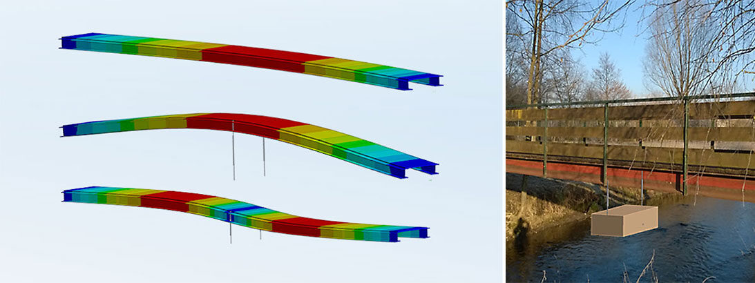
Let’s consider a slender pedestrian bridge where vibration amplitudes are too high when people walk across it. Say we want to reduce the most annoying vibration amplitude of the 2^nd mode, that is the 1^st vertical bending mode, by a pair of damping elements, and we are looking for the optimum damping coefficient c. A damped modal analysis does the job in Ansys Mechanical. The imaginary part of the resulting complex eigenvalues are the damped eigenfrequencies. Moreover, and even more interesting, the real part can be expressed in terms of a resulting modal damping ratio. The damping ratio ξ₂ of mode 2 is an excellent measure for the damping or the decay of the vibration of the whole bridge assembly.

A damping coefficient c close to zero yields the same result of ξ₂= 0 as we have obtained with the undamped solver. Increasing damping drastically soon is too much of a good thing. Again, the reported damping ratio for mode 2 is ξ₂ = 0. Now we have figuratively spoken an almost rigid damper pot e.g., filled with very viscous bitumen resulting in sort of a fixed support for the center of the bridge. After some trials we obtain a value of c = 10⁴ Ns/m for the optimal damping coefficient. As a result, we get a maximum damping ratio of ξ₂= 17% for the assembly. Please note: 17% is huge because we get an amplitude drop of 90% after only 2 cycles. From this simple example, we draw the following conclusions:

1. Known damping of a distinct component can be “translated” in damping of the full assembly mode by mode, an exciting result for the design of damping measures.
2. There is an optimum for each damping measure. The modal damping ratio, computed by means of damped modal analysis, is the suitable target variable, which virtually imposes itself for optimization.
3. Once the optimum damping coefficient has been determined, the next step is to consider how it could be realized technically, for example by simply purchasing the appropriate damping device from catalogue or by designing with strongly damping high-polymer materials oneself rendering the simulation model more detailed.

Damped modal analysis for a bridge with discrete damping measures looking for the optimal damping constant | © CADFEM

How to enter damping in Ansys Mechanical?

The most common way to enter damping is to simply open the analysis settings with its sub-branch damping controls. For many reasons mode superposition (MSUP) is the working horse of any dynamic analyst. Here, it is straight-forward to enter damping in terms of the well-known damping ratio ξ = c/c_cr = c/2mω as a fraction of critical damping, where no zero crossing of the deflection can be observed no more. For that case we have ξ = 1 = 100% whereas many practical structural assemblies can be assumed to have a damping ratio in the order of 1%. From definition it is already clear that the damping ratio cannot be a material parameter, since it depends on both the natural frequency and the mass of an oscillator.

Without any more detailed knowledge in the primary phase of the simulation of a new design it is usually pragmatic to take this value for granted for the whole assembly. For that purpose, we simply enter one damping ratio for the whole model as it is pointed out in the left figure where a damping ratio of ξ = 1% is assumed in a harmonic response analysis based on mode superposition – that’s it. Note that eigenfrequency ω must be available to define damping ratio ξ. We will come back to this issue in the next section. It is worth mentioning that this spread of damping over the whole model is called proportional damping because the damping matrix is assumed to be proportional to the global stiffness matrix.

But what’s if you cannot use MSUP for any reason? Say you must compute just 1 frequency point and you would have to compute hundreds of modes for MSUP to achieve this. In this case the method of FULL matrices might be much cheaper in terms of computational resources. Or maybe you must take care of frequency dependent material parameters which makes modal analysis impossible to do. Again, a FULL analysis is the method of choice despite the fact it is known to be much more expensive. Now you must enter loss factor η = 2·ξ= 2% in our example. Don’t forget this simple relation and please don’t enter any value carelessly just because anybody gave you a damping value expressed as an ambiguous percentage.

Analysis Settings with Damping Controls for MSUP (left) and FULL (right)  | © CADFEM

Closer to materials science – define loss factor

In a Harmonic Full analysis you must enter loss factor η because natural frequency ω and subsequently damping ratio ξ is not defined, then. For a MSUP analysis, on the other hand it is up to the user to decide about “Damping Define By” “Damping Ratio” or “Constant Structural Damping Coefficient” (the Ansys term for loss factor). But what is the definition of the loss factor? We can grasp the meaning when looking onto a stress-strain diagram for a material specimen. For a linear-elastic Hooke material we would simply have a straight line which is enclosing the blue triangle. This area is known to be the strain energy density U_ref stored in an elastic body due to deformation.

When repeating the stress-strain test for a linear viscous material specimen we will get the well-known hyseresis ellipsis, which is a clear indicator for damping. The area enclosed within the ellipsis corresponds to the energy dissipated during one cycle of vibration. This permits one to develop a physical meaningful definition of the loss factor η = W_Dh/2πU_ref. Thus, the loss factor indicates what fraction of the vibratory (reversible) mechanical energy is lost (i.e., converted into heat) in one cycle of vibration [Cremer1988]. This way the concept of the loss factor can be easily extended to arbitrary nonlinear dissipation mechanisms.

Another interpretation comes from the observed phase angle δ between stress σ and strain ε, which leads to the relation η = tan δ. Extraction of δ  by means of a DMA test (Direct Mechanical Analysis) is a prominent test method to determine the loss factor as a function of both frequency and temperature. Loss factor, not damping ratio is tabulated in most material science publications or textbooks on damping materials [Nashif1985]. For its usage in a simulation environment, we are not bound to knowledge of the eigenfrequency ω. Just the knowledge of the excitation frequency Ω is required. Thus both, harmonic FULL and MSUP analysis but not transient analysis can work with η.

Stress-strain hysteresis for a linear viscous and an arbitrary nonlinear material specimen  | © CADFEM

What are typical damping values?

Materials behave very different with respect to damping. For a first estimate it is helpful to have a rough picture of typical damping values. Metals like steel or aluminum typically show very low loss factors which are known to be constant over a wide range of frequencies and temperatures. On the other hand, high polymer materials bred for optimum damping properties show a significant dependency on frequency and temperature which must be considered when designing the optimum damping behavior. Vibration reduction for acoustic frequencies in the vicinity of a hot drive train has different requirements on the optimum material compared to the winding head of a fast-rotating textile machine at room temperature.

Metals hardly provide any notable damping. Damping of metal structures in many cases result from parasitic effects such as joint damping due to dry friction or displacement (pumping) of air/fluid in gaps or adjacent media, e.g., energy loss due to sound radiation. Often, one gets an overall idea of typical damping values for one's assembly by means of simple measurements of decay time or half-power bandwidth. The average of those values is typically entered as a global damping value for the entire assembly as shown above.

However, if highly damping materials are used for vibration reduction, it is worth to invest more care because those are the clue to success for remarkable vibration reduction and decide about speed, efficiency, output of your machine or on the other hand fatigue failure due to high resonant amplitudes. For proper input into simulation either you have got detailed material damping parameters from the manufacturer, or you characterize them by means of relevant test procedures like DMA offered by material testing offices and service providers. Is that worth the efforts? In any case, as we will see in the next section.

Typical loss factors for material classes:

How to tailor vibration reduction with damping material?

As we have seen it is not worth the trouble to set-up an own library of damping values for typical metallic materials due to their minor contribution to overall assembly damping. But if we really must address a resonance problem and if we can't get rid of the problem by any other approved engineering technique, then the great hour of damping design strikes. Either the problem is worth to develop an own design or finished, commercially available components or semi-finished products such as composite sheets with damping treatment are the method of choice.

Let’s investigate the latter for a moment because all required simulation techniques can be explained based on this very simple application. The damping properties of two metal cover sheets, say 1mm thick (η<<) can be significantly increased by inserting a thin viscous core like neoprene with 50µm and remarkable high η=0.28 for instance. Drive train and other automotive applications with the need for comfort (low vibrations, acoustics) can be addressed this way leading to much better damping properties compared to pure metal sheets. How to analyze a situation like that with a mix of materials with different damping properties ( → non-proportional damping)?

Again, damped modal analysis does the job. Now, however, damping is a material property to be entered in Engineering Data > Material Dependent Damping > Damping Ratio (Note: Constant Structural Damping Coefficient = loss factor η shown one line later for control purposes). This way after input of the known elastic and damping properties at material level the overall sandwich damping can be computed to be η=0.06 just to give an example. Note again: this η=0.06 is not an input value, this component loss factor is a simulation result answering your vibration or noise design problem! What is the maximum achievable damping for my component or assembly? What is the influence of layer thickness, material selection?

Constrained Layer Damping Treatment (CLDT) | © CADFEM

What else is possible in Ansys Mechanical?

We must conclude and cannot go more into details within this short article despite the fact that there are a lot more remarkable simulation chances when damping is no longer considered as the enemy of the simulation engineer but his friend. A list of “can be simulated” topics to mention a few:

• MSUP harmonic response for materials with distinct damping properties. MSUP for non-proportional damping as we clearly face here? Yes, this works efficiently by the reduced (QRDAMP) method projecting the damping matrix in modal subspace for instance.
• Viscoelastic material properties as a function of frequency, e.g. taken from DMA test report as the most accurate way to simulate high-damping materials.
• Rotating damping as a destabilizing parameter in rotordynamics.
• EHD oil film damping
• Added mass of an enclosed heavy fluid like water in a tank simulated by acoustic elements in Mechanical. By the way fluid mass, not damping from viscosity explains the reduction in vibration amplitude in this scenario.

You remember the pedestrian bridge example? Did you quietly think to yourself, no one would put a damper in the middle of the river here after all? Right, there are smarter techniques. The well-known problem after opening of the London Millenium Footbridge had been fixed by TMD (tuned mass dampers). Vibration isolation is another way to get rid of undesired vibrations. In both cases, vibration reduction primarily is a matter of stiffness, not damping. If you want to get more insight in all those phenomena and their simulation solutions a dedicated CADFEM training [Moosrainer 2022], also available as e-Learning lead you through step by step accompanied with a lot of practical exercises to get prepared to tackle own vibration reduction problems.

Vibrating pedestrian bridge with a sketched tuned mass absorber (TMD) | © CADFEM

Cover Images: Left: © CADFEM GmbH | Right: © CADFEM GmbH
First published: January, 2023

References
[Cremer1988] Cremer, L.; Heckl, M. and Ungar, E. E.: Structure-Borne Sound. Springer Verlag, Berlin, 2^nd edition (1988).
[Moosrainer2022] Moosrainer, M.: Understand and simulate damping of mechanical vibrations, CADFEM Seminar (2022).
[Nashif1985] Nashif, A. D.; Jones, D. I. G. und Henderson, J. P.: Vibration Damping. John Wiley & Sons, New York (1985).