‘All models are wrong, but some are very useful.’

As is so often the case in the world of simulation, certain effects can be calculated, or a ‘model’ exists to depict the desired effects. The model is a kind of black box that represents a shortcut for the given case, e.g. to save computing power and thus arrive at a meaningful statement from an engineering point of view with reasonable effort. Let’s first look at 3 scenarios:

1. Which fan is needed to operate the existing flue gas denitrification system? For denitrification, an impeller must be used that can handle the given process parameters (heat, pressure, humidity, ...); the geometry of the impeller is up for discussion and local effects are relevant. see Model: Passage (Fig 1).
2. Which fan does an enclosure need in order to sufficiently and efficiently cool the switching electronics inside? The availability of the fan is crucial; a ‘purchased part’ should be modelled and placed. The system behavior and the so-called ‘fan characteristic curve’ are important; local effects are relevant, e.g. to prevent hot spots. see Model: 3D Fan Zone (Fig 1).
3. Which fans need to be placed at which point in an underground car park or tunnel ceiling in order to ensure smoke extraction in the event of a fire, for example? The decisive factor here is to map the ‘displacement effect’ of the fans in order to predict the smoke gas distribution. The local effects on the fan itself do not play a role, only the ‘effect of the fan’ on its surroundings is relevant. see Model: 2D Fan Zone (Fig 1).

Let’s imagine that we have two rooms, A and B, which are connected to each other via a fan at the top and several ducts at the bottom. The question now is, what results do our fan models deliver at a given rotational speed for this exemplary case?

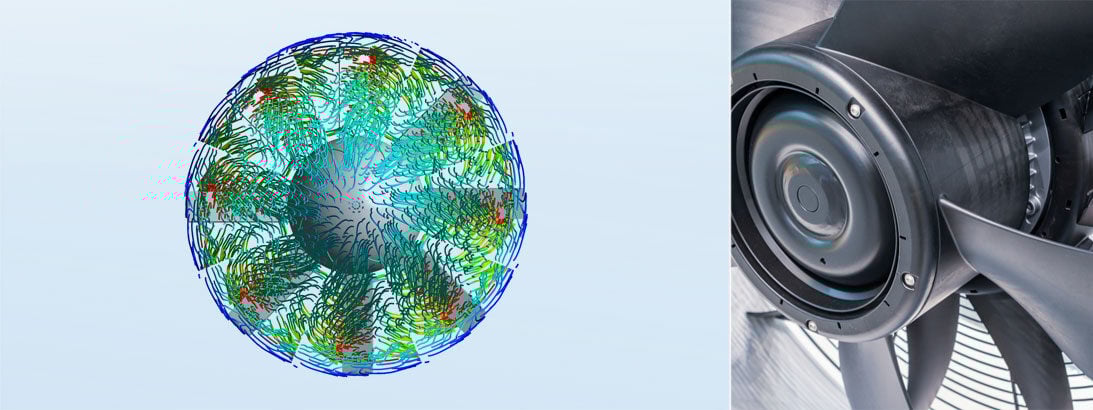
Fig. 1a: Exemplary fan including intake and outtake area, installed between ‘rooms’ A and B | © CADFEM

Fig. 1b: Impeller with the model volumes for passage, 3D and 2D Fan Zone | © CADFEM

Fan calculation with one passage

When you imagine a fan, you can identify a repeating geometry for many applications in the ‘rotating fluid area’ based on the number of ‘blades’ - the so-called passage. If you have this geometry available, you can use this fan in a stationary simulation based on the rotor speed, for example, to fully calculate the interaction with an overall system with all the desired effects. The core idea is that the passage is repeated around the circumference, so the stationary environment sees a ‘multiple’ of this passage (see Fig. 2). Instead of the 360° geometry, only one sector with periodic boundaries is used.

At the transition from the stationary to the rotating system, a so-called General Turbo Interface (GTI) is used so that the rotating zone can communicate with the stationary zone; the only direct input is the rotational speed. All effects resulting from the impeller rotation are fully calculated. For example, the actual intake behavior, the acceleration over the passage and the swirl-induced wake are fully mapped. In this way, detailed analyses of the blade flow and wake can be carried out and corresponding improvements to the blade contour, the blade angle or the blade root can be derived.

The high level of detail offered by the GTI comes at a certain price. The necessary resolution of the blade geometry and the general calculation process place increased demands on the computing resources and the computing time. In addition, the geometry of the impeller must be available, which is not always the case, especially with purchased parts.

Fig. 2a: Fluent’s Turbo Mode allows the single passage to be connected sensibly and correctly to the far field (rooms A and B) | © CADFEM

Fig. Single passage with periodic edges; the full model of the original "full" fan wheel is indicated | © CADFEM

The kernel of the fan – The 3D Fan Zone

If we imagine the swept area of the impeller blades as a donut (Figure 3, right), we can see that the flow in this area is accelerated by the fan according to the direction of rotation and impeller geometry. We can therefore replace the fan with an impulse source that lies within the donut area. The so-called 3D Fan Zone takes up precisely this idea and translates certain fan characteristics into the appropriate momentum source in the radial, tangential and circumferential directions. The 3D Fan Zone is therefore able to reproduce the contribution of a fan to the surrounding fluid; it also maps the downstream swirl.

The necessary inputs are the local coordinates of the ‘fan’, the basic impeller dimensions, and the fan inlet area. With the 3D Fan Zone, much has already been done correctly and various scenarios can be correctly mapped and analyzed: Different speeds, start-up behavior and overrun interaction. For example, several fans can interact with each other as an ensemble and the respective fan wake behavior can be mapped in detail (e.g. no flow in the hub area). Basic information about the rotor must be known but not resolved geometrically.

Fig 3: The swept fan volume in blue and the zone setting for the 3D Fan Zone. | © CADFEM

Turn 3 into 2 - The 2D Fan Zone

If you now take the final step and are not at all interested in the local distribution inside the fan, then only the fact that something has happened via the fan inlet to its outlet is relevant - the pressure has increased. This final simplification requires the swirl from the fan to be specified explicitly or in the form of coefficients. Here, too, a characteristic curve can be specified instead of a constant pressure jump (axial direction). What is needed is a disc in place of the fan wheel and the desired pressure increase (see Fig. 4).

This is an ‘internal’ cut through the calculation area, in which we manipulate the fluxes crossing over these control surfaces by directly applying the required momentum. In analogy to the 3D fan zone, the sources are now located on one surface and are no longer distributed in space. We ‘merge‘ a pressure outlet directly back to a pressure inlet - in the same place.

If we now place this 2D Fan Zone at the border of our flow volume we obtain the corresponding intake fan and exhaust fan boundary conditions. Fan characteristics can also be specified here and, for example, housings or ventilation systems can be designed.

Fan Fact: The fan boundary conditions for inlet and outlet fans described in this section are also available in Ansys Discovery, where they are already provided with an extensive manufacturer list of fan characteristics. This compendium can therefore be used, for example, to select a suitable standard fan for a given task and geometry.

Fig. 4: The 2D Fan Zone as a boundary condition. The selected surface must represent a section in the calculation area and must therefore be meshed/imported with the internal type | © CADFEM

Full 3D or sliced up?

As can be clearly seen in Figure 5, the influences based on the selected fan model are sometimes clear but localized. In the case of the passage, for example, the flow clearly clings to the wall in the wake, but not in the case of the 3D Fan Zone; in this case, a separation occurs at the trailing edge. In the case of the 2D Fan Zone, the flow attaches to the wall again due to the selected tangential and radial velocities. In all cases, however, the characteristics of the inflow are similar.
Conclusion on the ‘designed’ fan geometry: A shaft with boards conveys air, but not very efficiently. There is still room for improvement here.

What do you do with your next fan? Do you select a suitable fan directly from the manufacturer list and use Ansys Fluent or Ansys Discovery to calculate the local flow and temperature influences via the 2D Fan Zone? Or do you calculate the corresponding performance and flow control in your overall system for a parametric impeller geometry, including all internals and guide vanes? As a passage or as a complete impeller in a transient simulation?

Not quite a ‘fan’ yet? Get in touch and we can showcase Ansys Discovery directly using your ventilation system in a live demo.

Fig.  5: Comparison of the local flow distribution near the fan (0.0 - 2.0 m/s, 500 RPM). The dimensions and the pressure build-up from the passage were approximated for the 2D and 3D fan zones | © CADFEM

Cover images: Left: © CADFEM GmbH | Right: © Adobe Stock