Understanding the Operating Noise of Electric Motors
Jürgen Wibbeler
16.01.2026
TechArticle 26/1 | Multidisciplinary Simulation from Electromagnetics to Acoustics
While writing this text, my laptop is practically silent. Only when it works hard does it blow warm air out with noticeable noise. Twenty years ago, things were different: fans and hard drives were constantly humming under the desk. Today, rotating drives have almost disappeared, and even the fans are barely audible.
Noise-inducing vibrations in an electric motor | © CADFEM / Adobe Stock / ID: MJ5HEE
Conclusion
- Identify noise sources: Electric motors generate tonal and broadband noise through magnetic air-gap forces. These act periodically in time and space and shape the acoustic behavior.
- Use simulation: Ansys Maxwell and Motor-CAD capture air-gap forces, which are transferred to Ansys Mechanical for harmonic response and acoustic simulations – making resonances and noise development visible.
- Enable optimization: The workflow from electromagnetics to acoustics predicts and reduces motor noise. Ansys Sound adds psychoacoustic evaluations and listening tests for practical improvements.
Where Do the Tones Come from?
An electric drive system contains various noise sources. It starts with the rotating field in the motor and its magnetic air-gap forces, which excite vibrations at the stator and housing and can cause torque oscillations at the rotor. Fan noise counts as flow noise and is usually broadband, while electric motors often produce tonal vibrations at specific frequencies, called temporal orders. These occur as multiples of the rotational speed and depend on motor design, such as pole and slot count. Commutators and inverters enrich the spectrum with additional, often dominant frequencies. Even weak tonal noise can be very disturbing compared to broadband noise in everyday life.
To predict and reduce motor noise, you must start with the air-gap forces between rotor and stator. Both Ansys Maxwell and Ansys Motor-CAD allow recording these forces as functions of rotor angle or time from FE simulation. Their structure is worth examining to better understand vibration excitation. Air-gap forces are not only periodic in time but also in space. Cyclic force density patterns form around the air-gap circumference. They contain different wave numbers on the full circle, called spatial orders.

Magnetic field calculation with Ansys Maxwell: Field lines of a four-pole permanent magnet motor (left) and force density vectors on the stator around the air-gap circumference (right) | © CADFEM / ID:P4A9WV
The image shows four distinct maxima of force density, corresponding to the 4th spatial order. Additional orders, which are not easily visible, can be determined through Fourier decomposition. Each stator responds differently to the various spatial orders in the excitation and exhibits very different resonance frequencies. A successful motor design will now avoid having these orders excite sensitive resonances of the stator and the housing within the motor’s operating range.
How Does the Structure Respond to Excitation?
Air-gap forces can already provide important clues as to whether you are potentially designing a “noise maker.” Comparative better-worse analyses of the electromagnetically active part are possible in any case. However, to obtain the resulting vibration on the exposed housing surface and then calculate up to airborne sound radiation, the air-gap forces are coupled in the frequency domain into a structural-dynamic harmonic response analysis. Between Ansys Maxwell or Motor-CAD and Ansys Mechanical, there is a prepared XML-based interface for this purpose.
Code:
# import libraries
import os
from ansys.geometry.core import launch_modeler_with_discovery
# create string with discovery code
cmd = """
# fix Small Faces with a smaller width of 1.5 mm
FixSmallFaces.FindAndFix(FixSmallFacesOptions(Width=MM(1.5)))
# define variables
bending_face = None
z_bending_face = float('inf')
# loop through faces
for face in GetRootPart().Bodies[0].Faces:
# get z coordinates and shape
z_cordinates = face.EvalMid().Point.Z
shape = face.Shape.Geometry.ToString()
# get bending face on the bottom
if (shape.Contains("Cylinder")):
if(z_cordinates < z_bending_face):
z_bending_face = z_cordinates
bending_face = face
# […] identify other important faces (clamping faces for example)
# save the faces in named selections
Selection.Create(bending_face).CreateAGroup("bending_face")
# […] also save other faces in named selections
"""
# create a text file and input the discovery code
fd = os.getcwd()
path = os.path.join(fd, "discovery.py")
with open(path, "w", encoding="utf-8") as file:
file.write(cmd)
# start discovery, open the geometry and run the code
modeler = launch_modeler_with_discovery(product_version = 251, hidden = True)
design = modeler.open_file(os.path.join(fd,"geometry.step"))
modeler.run_discovery_script_file(os.path.join(fd,"discovery.py"))
# save the finished geometry and delete the code file
design.save(os.path.join(fd,"geometry_prepared.scdocx"))
modeler.close()
os.remove("discovery.py")
Code:
# import libraries
import os
import ansys.meshing.prime as prime
from ansys.meshing.prime.graphics.plotter import PrimePlotter
# start client and assign lucid meshing
prime_client = prime.launch_prime()
model = prime_client.model
mesh_util = prime.lucid.Mesh(model=model)
# define path to geometry
fd = os.getcwd()
input_file = os.path.join(fd," geometry_prepared.dsco ")
# create a surface mesh
mesh_util.read(file_name=input_file)
mesh_util.surface_mesh(min_size=2.0)
# create a volume mesh and display
mesh_util.volume_mesh()
display = PrimePlotter()
display.plot(model, update=True)
display.show()
# save mesh
mesh_file_cdb = os.path.join(fd, "mesh.cdb")
mesh_util.write(mesh_file_cdb)

Transfer of tooth forces and moments from the electromagnetic to the structural-dynamic simulation | © CADFEM / ID: UTZ6R6
From the mechanical surface vibration, the structure-borne sound level can be directly derived as Equivalent Radiated Power (ERP) in the spectrum. The entire workflow can be executed in speed steps over a speed range as a run-up simulation. In a so-called waterfall diagram, vibration and acoustic spectra are visualized over speed. Resonance peaks in the waterfall diagram reveal which temporal order hits a mechanical resonance frequency at which speed. For example, at 4500 rpm, the 24th order (1800 Hz) excites the housing torsional resonance. At 7000 rpm, the 32nd temporal order (3733 Hz) excites the fourfold eigenmode of the stator and housing. The cause is the 4th spatial order in the air-gap forces, which interacts with this eigenmode to the detriment of acoustic behavior.

ERP-waterfall diagram of a harmonic analysis for a run-up in Ansys Mechanical and examples of vibration modes at two selected resonances; Each line in the diagram represents the structure-borne sound level caused by a temporal excitation order (4, 8, 12, …) along the rotational speed | © CADFEM / ID: O4LXZY
Whitepaper
Correlation of the FE Model with the Real World
For structural-dynamic simulation, it is crucial that the eigenmodes and eigenfrequencies of the FE model match reality as closely as possible. Many model parameters, such as contact stiffness of joints, are vague or largely unknown.
The parametric correlation of an FE model with an experimental modal analysis (EMA) using the NVH Toolkit in Ansys Mechanical and Ansys optiSLang is described in a White Paper.
Request WhitepaperAnd What Does It Sound Like?
More precise results on radiated power and the spatial distribution of sound pressure level (SPL) are provided by a connected harmonic acoustics analysis of the sound field. A key result of the airborne sound analysis is a lower actual radiated power than indicated by the structure-borne sound level ERP. For the example data point 4500 rpm and 1800 Hz, the ERP value is 82.5 dB, while the airborne sound analysis calculates only 74.3 dB as radiated power (Sound Power Level). The reason are phase-related cancellations in the sound field (“acoustic short circuit”), which are not considered in the ERP value.
Code:
# import libraries
import os
from ansys.dpf import core as dpf
# open result file
fd = os.getcwd()
model = dpf.Model(os.path.join(fd,"result.rst"))
# get results and mesh
results = model.results
mesh = model.metadata.meshed_region
# extract displacement results
displacements = results.displacement()
field = displacements.outputs.fields_container()
# export the displacement field
my_export = dpf.operators.serialization.vtk_export()
my_export.inputs.file_path.connect(os.path.join(fd,"displacement.vtk"))
my_export.inputs.fields1.connect(field)
my_export.inputs.mesh.connect(mesh)
my_export.run()
# shutdown all dpf servers
dpf.server.shutdown_all_session_servers()

Acoustic sound field (sound pressure level) of the housing torsional vibration at 4500 rpm, 1800 Hz: contour plot and polar diagram in the plane perpendicular to the motor axis | © CADFEM / ID: 46PU50
It is obvious and easy to generate a sound for listening from the calculated ERP or SPL spectra. In fact, WAV files can be exported directly from Ansys Mechanical. However, such simulated motor noise usually sound very “sterile.” The perception of an emitted noise is strongly influenced by the transmission path to the ear and by incidental background noise. A simple tool for mixing calculated and measured sounds, applying transfer frequency response functions, or processing them otherwise is Ansys Sound – Analysis and Specification (SAS).
Psychoacoustic metrics of the noise can also be determined with SAS according to various standards. Take part in the Ansys Sound Training and learn – or hear for yourself – the effects of layout changes on subjective acoustics. This way, you’ll get much closer to real perception.
Ansys Fluent GPU Performance Testing – Use Case
Ob im Maschinenbau, in der Luftfahrt oder bei der Produktentwicklung: Strömungssimulationen sind für präzise und schnelle Entwicklungsprozesse unerlässlich. Doch wie unterscheiden sich CPU- und GPU-basierte Simulationen, und was sind die wichtigsten Kriterien bei der Hardwarebewertung? Dieser Beitrag beleuchtet grundlegende Unterschiede, Leistungsmetriken und die Anwendungsmöglichkeiten von GPU- und CPU-Setups für Ihre CFD-Projekte.t
Reading Is Silver, Listening Is Gold
Minimizing sound radiation has become a core topic in the development of electric drives. That’s why you no longer hear humming and singing from notebook cooling, and many other electrical devices have become quieter. Ansys tools support the necessary analyses and selective measures. With electromagnetic, structural-dynamic, and acoustic simulation and the required interfaces, a seamless calculation process for motor noise is available.
Within Ansys Workbench, this process is even fully integrated. Electromagnetic simulation (Ansys Maxwell 2D or 3D), harmonic response analysis (Ansys Mechanical), and harmonic acoustics analysis (Ansys Mechanical) are placed in a Workbench project and graphically linked. The internal project logic then transfers the data from one module to the next.

Integrated simulation workflow from electromagnetics to acoustics in Ansys Workbench | © CADFEM / ID: CI6FXE
In the Noise Computation for Electrical Drives training, you will learn how to use this workflow in practice to understand noise generation in your electric machines and identify optimization potential. If your application involves not only the electric machine itself but also gears and bearings, watch out for the next TechArticle in this series on noise generation in machinery …
More on the Topic
-
Bringing Simulation Models to Life with Ansys Sound

Discover the quality of the sound generated by your virtual products and learn how to assess this in terms of psychoacoustic criteria
-
Noise Computation for Electrical Drives

Learn how to calculate the electromagnetically induced vibration and noise emitted by electric motors using Ansys tools.