PyAnsys: The Key to Workflow Automation
Moritz Weißenbäck
05.12.2025
TechArticle 25/11 | Successful Automation of Simulation – a Practical Example
Manual processes often characterize the everyday work of Ansys Mechanical users in simulation and calculation. However, automation offers enormous opportunities, saving time, creating standards, and ensuring quality. Using a concrete practical example, I will show you step by step how automation can be successfully implemented.
Various bending tools clamped in place and successive simulation steps show | © CADFEM (Austria) GmbH
Summary
- Recurring, manual FEM simulations for bending tools are to be replaced by an automated workflow that processes geometry and machine data and automatically generates reports.
- Use of various Python libraries (including PyGeometry, PyPrimeMesh, PyMAPDL, PyDPF-Core, PyD-ynamicReporting) for geometry preparation, meshing, simulation, evaluation and report generation in a continuous process.
- Structured automation in three steps: Create named selections, replicate the existing simulation process using a script, and evaluate and automatically document the results.
Motivation for Automation at Trumpf
Let's start with a practical example. Trumpf manufactures bending tools and simulates their stress. Due to the many different tools, the repetitive simulation process, and high-quality standards, automation is an excellent solution here. The goal is to develop a workflow that automatically generates a calculation report using geometry and machine data as input.
The solution: PyAnsys. PyAnsys is a collection of Python libraries for interacting with the Ansys product range. There are Python counterparts for almost all Ansys software products. For example, PyMechanical enables Python-based control of Ansys Mechanical. The PyAnsys libraries are freely accessible and usable, but it should be noted that a valid Ansys license is required to interact with certain software products. Detailed information on the individual modules and numerous examples can be found on the PyAnsys website.
Back to the project: how do you tackle such an extensive task? As with FEM, which breaks down complex problems into small solvable elements, it is advisable to divide the overall scope into manageable packages. The following steps are necessary:
- Prepare the geometry
- Perform setup and solving
- Evaluate results and create report
These tasks can be efficiently automated with the appropriate PyAnsys modules. The direct interaction between the individual modules creates a continuous workflow. In the next section, we will take a closer look at the individual steps.

Representation of input and output definition of the bending tool workflow from Trumpf | © CADFEM (Austria) GmbH
Geometry Preparation with Ansys Discovery
As with manually created simulations, the geometry is the starting point. The key to successful automation lies in a uniform and structured approach – especially in the preparation step of the geometry. A central element here are the so-called named selections, which allow relevant geometry areas to be grouped and clearly named. Therefore, the number of edges or surfaces in a geometry to which a load is applied does not matter, as only the named selections are used in further processing. Boundary conditions or loads can be applied directly to these named areas. This makes the workflow much more efficient, as subsequent modules can access these named areas in a targeted manner and different geometries can be uniformly processed.
Named selections can be easily created with Ansys Discovery. In the software's scripting editor, bodies, surfaces or edges can be selected and saved based on rules – for example, based on their position, shape, orientation or size. The challenge here is to develop an algorithm that automatically recognizes the relevant bodies and faces for each geometry. The routine developed in Ansys Discovery can be copied directly as text and called up using the PyGeometry library. The simplified code below shows how two surfaces are being selected on the bending tool and saved in a named selection.
-
Code
# import libraries
import os
from ansys.geometry.core import launch_modeler_with_discovery# create string with discovery code
cmd = """
# fix Small Faces with a smaller width of 1.5 mm
FixSmallFaces.FindAndFix(FixSmallFacesOptions(Width=MM(1.5)))# define variables
bending_face = None
z_bending_face = float('inf')# loop through faces
for face in GetRootPart().Bodies[0].Faces:# get z coordinates and shape
z_cordinates = face.EvalMid().Point.Z
shape = face.Shape.Geometry.ToString()# get bending face on the bottom
if (shape.Contains("Cylinder")):if(z_cordinates < z_bending_face):
z_bending_face = z_cordinates
bending_face = face# […] identify other important faces (clamping faces for example)
# save the faces in named selections
Selection.Create(bending_face).CreateAGroup("bending_face")
# […] also save other faces in named selections
"""# create a text file and input the discovery code
fd = os.getcwd()
path = os.path.join(fd, "discovery.py")
with open(path, "w", encoding="utf-8") as file:file.write(cmd)
# start discovery, open the geometry and run the code
modeler = launch_modeler_with_discovery(product_version = 251, hidden = True)
design = modeler.open_file(os.path.join(fd,"geometry.step"))
modeler.run_discovery_script_file(os.path.join(fd,"discovery.py"))# save the finished geometry and delete the code file
design.save(os.path.join(fd,"geometry_prepared.scdocx"))
modeler.close()
os.remove("discovery.py")
Code:
# import libraries
import os
from ansys.geometry.core import launch_modeler_with_discovery
# create string with discovery code
cmd = """
# fix Small Faces with a smaller width of 1.5 mm
FixSmallFaces.FindAndFix(FixSmallFacesOptions(Width=MM(1.5)))
# define variables
bending_face = None
z_bending_face = float('inf')
# loop through faces
for face in GetRootPart().Bodies[0].Faces:
# get z coordinates and shape
z_cordinates = face.EvalMid().Point.Z
shape = face.Shape.Geometry.ToString()
# get bending face on the bottom
if (shape.Contains("Cylinder")):
if(z_cordinates < z_bending_face):
z_bending_face = z_cordinates
bending_face = face
# […] identify other important faces (clamping faces for example)
# save the faces in named selections
Selection.Create(bending_face).CreateAGroup("bending_face")
# […] also save other faces in named selections
"""
# create a text file and input the discovery code
fd = os.getcwd()
path = os.path.join(fd, "discovery.py")
with open(path, "w", encoding="utf-8") as file:
file.write(cmd)
# start discovery, open the geometry and run the code
modeler = launch_modeler_with_discovery(product_version = 251, hidden = True)
design = modeler.open_file(os.path.join(fd,"geometry.step"))
modeler.run_discovery_script_file(os.path.join(fd,"discovery.py"))
# save the finished geometry and delete the code file
design.save(os.path.join(fd,"geometry_prepared.scdocx"))
modeler.close()
os.remove("discovery.py")
Bonus tip: Ansys Discovery is not only suitable for creating named selections, but also for geometry editing and modeling additional geometric elements. The recording function, which translates manual actions in the software directly into Python code, is very helpful for programming. For further in-depth information, I recommend checking out the following two trainings: Geometry Preparation in Ansys Discovery and Automation with Ansys Discovery Scripting.
Executing the code in Discovery with PyGeometry | © CADFEM (Austria) GmbH
PyPrimeMesh & PyMAPDL: From Mesh to Simulation
What happens after geometry preparation? Generally, a manually set up simulation is already availa-ble, as is the case at Trumpf. This serves as a template for subsequently reproducing and automating the process. There are two approaches available for structural problems:
- Interaction with Mechanical via PyMechanical – similar to Discovery, the recording function can be used to automatically generate the appropriate Python code and embed it directly. This method is particularly suitable for users who are already familiar with Ansys Mechanical. A detailed introduction is provided in the technical article ‘First steps with PyAnsys using an end-to-end example’.
- Use of MAPDL via PyMAPDL – we will opt for this variant here. However, before we venture into set-ting up the simulation in MAPDL, a mesh is first generated from the geometry. The PyAnsys library PyPrimeMesh is ideal for this purpose. Below is a small, simple demo code that can be used to mesh the geometry quickly and efficiently.
-
Code
# import libraries
import os
import ansys.meshing.prime as prime
from ansys.meshing.prime.graphics.plotter import PrimePlotter# start client and assign lucid meshing
prime_client = prime.launch_prime()
model = prime_client.model
mesh_util = prime.lucid.Mesh(model=model)# define path to geometry
fd = os.getcwd()
input_file = os.path.join(fd," geometry_prepared.dsco ")# create a surface mesh
mesh_util.read(file_name=input_file)
mesh_util.surface_mesh(min_size=2.0)# create a volume mesh and display
mesh_util.volume_mesh()
display = PrimePlotter()
display.plot(model, update=True)
display.show()# save mesh
mesh_file_cdb = os.path.join(fd, "mesh.cdb")
mesh_util.write(mesh_file_cdb)
Code:
# import libraries
import os
import ansys.meshing.prime as prime
from ansys.meshing.prime.graphics.plotter import PrimePlotter
# start client and assign lucid meshing
prime_client = prime.launch_prime()
model = prime_client.model
mesh_util = prime.lucid.Mesh(model=model)
# define path to geometry
fd = os.getcwd()
input_file = os.path.join(fd," geometry_prepared.dsco ")
# create a surface mesh
mesh_util.read(file_name=input_file)
mesh_util.surface_mesh(min_size=2.0)
# create a volume mesh and display
mesh_util.volume_mesh()
display = PrimePlotter()
display.plot(model, update=True)
display.show()
# save mesh
mesh_file_cdb = os.path.join(fd, "mesh.cdb")
mesh_util.write(mesh_file_cdb)
Once the mesh is available, you can start creating the APDL code. The development environment for this is Mechanical APDL, also known as Ansys Classic. A small tip: The code does not have to be cre-ated entirely manually, as an input file can be generated in Workbench and then customized. Once the setup and solving in MAPDL are working as desired, the code is transferred to Python. The following function is useful here:
from ansys.mapdl import core as pymapdl
pymapdl.convert_script("mapdl.mac","mapdl.py")

Mesh created with PyPrimeMesh | © CADFEM (Austria) GmbH
Result Processing with PyDPF Core
Once the simulation has been successfully completed, the results are available in the result file. The Python module PyDPF-Post is suitable for simple post-processing tasks. However, if more complex evaluations of entire result fields are to be carried out, it is advisable to use the more comprehensive PyDPF-Core library. This allows efficient and powerful workflows to be created. A simple example of how to export the displacement results as a vtk file (3D model) is shown below:
-
Code
# import libraries
import os
from ansys.dpf import core as dpf# open result file
fd = os.getcwd()
model = dpf.Model(os.path.join(fd,"result.rst"))# get results and mesh
results = model.results
mesh = model.metadata.meshed_region# extract displacement results
displacements = results.displacement()
field = displacements.outputs.fields_container()# export the displacement field
my_export = dpf.operators.serialization.vtk_export()
my_export.inputs.file_path.connect(os.path.join(fd,"displacement.vtk"))
my_export.inputs.fields1.connect(field)
my_export.inputs.mesh.connect(mesh)
my_export.run()# shutdown all dpf servers
dpf.server.shutdown_all_session_servers()
Code:
# import libraries
import os
from ansys.dpf import core as dpf
# open result file
fd = os.getcwd()
model = dpf.Model(os.path.join(fd,"result.rst"))
# get results and mesh
results = model.results
mesh = model.metadata.meshed_region
# extract displacement results
displacements = results.displacement()
field = displacements.outputs.fields_container()
# export the displacement field
my_export = dpf.operators.serialization.vtk_export()
my_export.inputs.file_path.connect(os.path.join(fd,"displacement.vtk"))
my_export.inputs.fields1.connect(field)
my_export.inputs.mesh.connect(mesh)
my_export.run()
# shutdown all dpf servers
dpf.server.shutdown_all_session_servers()
However, significantly more complex workflows can also be implemented – such as calculating the utilization rate in accordance with the FKM guideline, as implemented by Trumpf, for example.
Finally, the step of report generation is still missing. For this purpose, the PyDynamicReporting library can be used, which is particularly suitable if PyMechanical has been used previously. It allows report templates to be created quickly and easily and automatically filled with content. Alternatively, reports can be created manually – for example, as HTML files – using any modules from the Python world. Interactive 3D result plots can also be integrated here, enabling further analysis directly in the report.

Displacement results in mm of the vtk model | © CADFEM
The Automation Recipe for Simulations
For those encountering this subject for the first time in this article, this is probably quite a lot of new information. For this reason, let's summarize the most important steps:
- Step 1: All geometric elements required in the simulation – such as a surface to which a force is applied – should be saved as a named selection. The assignment can be carried out in Discovery based on specific rules.
- Step 2: Use an existing manual simulation process as a basis and then use PyMechanical or PyMAPDL to reproduce the workflow in automated form. Develop the codes step by step in the respective development environment (Mechanical Scripting Editor or Ansys Classic), test them there and then transfer the individual code snippets to your Python environment.
- Step 3: For further analysis or post-processing, PyDPF-Core can be used to create customized workflows. The final step is report generation. For this, you can either use the PyDynamicReporting library or manually create an HTML file, in which interactive 3D result plots can also be integrated.
You now have a recipe that you can use to get started right away. The code examples shown are just simplified excerpts. However, they serve as a solid starting point. To automate your own tasks – as Trumpf has done – all you need to do is expand them to meet your specific requirements. At this point, I would like to refer you once again to the PyAnsys website, which provides many more examples. The training course Introduction to Python for Ansys also offers a good introduction to the topic. You now have all the tools you need to automate your workflows and avoid time-consuming, repetitive work. I wish you lots of fun and success with the implementation!

Recipe for automating a workflow with PyAnsys | © CADFEM (Austria) GmbH
Training Tip
Python Primer for Ansys
In this training, you will learn the basics of Python programming for using PyAnsys and automating your Ansys simulations.
Ansys Fluent GPU Performance Testing – Use Case
Ob im Maschinenbau, in der Luftfahrt oder bei der Produktentwicklung: Strömungssimulationen sind für präzise und schnelle Entwicklungsprozesse unerlässlich. Doch wie unterscheiden sich CPU- und GPU-basierte Simulationen, und was sind die wichtigsten Kriterien bei der Hardwarebewertung? Dieser Beitrag beleuchtet grundlegende Unterschiede, Leistungsmetriken und die Anwendungsmöglichkeiten von GPU- und CPU-Setups für Ihre CFD-Projekte.t
More on the Topic
-
Geometry Preparation in Ansys Discovery

Whether you work with Ansys Discovery or Ansys SpaceClaim, this training will teach you everything you need to know about modeling for Ansys.
-
Automation with Ansys Discovery Scripting

In this training course, you will learn to control Ansys Discovery via the script language Python: from geometry to simulation.
-
First Steps with PyAnsys using an End-to-End Example

In this article you will get an overview of the PyAnsys world as well as a short introduction on how to minimize the obstacles associated with automating your own Ansys simulations.