Which is the correct welding speed?

Welding processes generate a lot of heat output in the smallest possible area, which is why adapted process control is important in order to avoid defects and reduce welding beads - especially those on the forehead. Find out here why 5 mm/s is the right speed for this application and how it could be even faster.

Hero_Schweissen_1093x410

A lot of power in a small space

Welding processes are classic intermediate steps in the value chain in the metalworking industry (and meanwhile also for non-metals). The variants are diverse and range from electron beam welding in (almost) vacuum to laser welding or exotic methods such as friction welding and various atmospheres in MIG/MAG welding to electrode welding. However, the aim is the same: to melt material in a “focused” manner. The liquid material can either be easily removed (cutting) or it joins surrounding material (joining). And it is precisely this “focus” that ultimately determines the quality of the process.

As conventional and historically established as the process itself is, the physics involved with interactions between temperature and mechanics is just as complex: Weld distortion - also or especially in multi-layer welding -, weld pool formation, heat-affected zones, microstructural transformation, etc. Everything influences each other and, to make matters worse, non-linearly. Particularly with safety-relevant components or highly automated processes, a process design based on the motto “it will probably hold” is somewhere between “questionable” and “grossly negligent”. Simulation models can be used to generate much more substantiated statements about the process.

In this article, we want to look at how a continuous welding process can be analyzed, designed and, at best, even improved in a thermal simulation model. To do this, we use a little trick and transfer the real process with its movement and time dependency into a stationary simulation - this simplifies the evaluation and, above all, minimizes the calculation time. Ultimately, this results in the maximum permissible welding speed so that a sufficient weld seam quality is achieved and the highest possible productivity is reached.

TEASER~3

Negligence in safety matters | © Getty Images

Minimal principle: Achieve a lot with little effort

In addition to the purely thermal and structural-mechanical properties, a third factor comes into play: movement. In most cases, the welding source and the material to be welded move relative to each other. The temperature field is therefore not only dependent on the material properties, but also on the relative movement. At this point at the latest, it becomes clear that a calculation using analytical approaches and thumb formulas can only inadequately reflect reality.

However, we want to simplify the task for initial analyses and try to gain as much knowledge as possible with as little effort as possible. Therefore, the (laser) focus is initially placed on purely thermal simulations. The calculated temperature profile is often sufficient to make initial estimates of the mechanical results (stresses, deformations). These do not necessarily provide quantitatively correct results, but tendencies and worst-case scenarios can already be qualified.

One of the first steps in the development of a simulation model is to create the geometry. Nowadays, there is a bunge of tools available for this purpose, each of which differs in terms of appearance, operation and range of functions. The example under consideration was created in Ansys Discovery and represents a rudimentary Y-seam, which is partially filled by a submerged arc process. The weld head itself is represented by an applied heat output onto the welded joint that exists afterwards. In addition to the geometry, every simulation model also requires boundary conditions, loads and material data, which in our case have special features ...

TechArticle_Temperaturfeld_mit_Vorschub_Schweissprozesse-Temperaturfeldsimulation

Stationary temperature field simulation with mass transport | © CADFEM

Common characterization of solid and liquid

As an example, we use thermal data of a structural steel with a thermal conductivity of 60 W/mK, a density ρ of 7850 kg/m³ and a special heat capacity cp, which energetically takes into account the phase change between solid and liquid. This cp is stored as a function of temperature and is significantly increased in the melting temperature range. In reality, this increase in capacity only affects a very small temperature range. For numerical reasons, however, the range is widened. This is where the usual compromise in simulation comes into play: in order to take into account the effect of a very narrow temperature band, you need a lot of elements and therefore a lot of patience.

The procedure can be illustrated using figures: We initially assume a constant heat capacity of 434 J/kgK. This should now apply up to 1500°C, where melting begins. The material is then completely melted at 1600°C. The enthalpy of fusion of iron is 275,000 J/kg. Consequently, an energy requirement of 434 J/kgK * 100 K + 275,000 J/kg = 318,400 J/kg is required from the start of melting to the completely liquid state. This requirement is in turn distributed over the relevant temperature range and results in a heat capacity of 3184 J/kgK. In practical terms, this means that a temperature change in this range requires (heating up) or releases (cooling down) much more energy.

Let's remember: We define cp and ρ and talk about TEMPORARY temperature changes when passing through a phase change in a STATIONARY model... strange, isn't it? The background is that an advection term is usually ignored in the usual notation of the heat conduction equation, because continuous movements are as rare as the “en passant” move in chess. However, the simulation recognizes this term and therefore allows movement in the stationary case. For the sake of completeness, in case it should ever be relevant: Mass transport could also be considered in the same way in transient analyses.

TECHAR~2

Material data with transformation enthalpy | © CADFEM

Movement at a standstill

Even if the simulation model is intended to represent a continuous process, the modeled geometry is initially limited. To describe the simulation process, the temperature at the imaginary entry point of the material should be provided with a temperature boundary condition. If no machining step took place before the heating process, it makes absolute sense to apply the ambient temperature here. If a transient heating process is also considered for this application, the temperature boundary condition could be dispensed with and such a transient simulation could be used to determine how long it takes to reach the steady state.

The classic thermal boundary conditions (convection, radiation, temperature at the material inlet) are used for our simulation. Nothing special so far. However, the process becomes really interesting when a mass transport effect is implemented. This requires three tricks. The mass transport option is reserved for linear thermal elements. Therefore, the corresponding bodies must be meshed with elements without center nodes. Next, the components require the key option no. 11 to be switched to the value 1 and a definition of so-called real constants. If only one element type is used, the two lines from the illustration are sufficient.

And the third trick is to assign a speed to the associated calculation nodes using an APDL code. The speed of 5 mm/s in the y-direction must be defined in relation to the global Cartesian coordinate system. This in turn means that for rotational movements, which in the worst case do not even run around one of the coordinate axes, it is necessary to fall back on long-forgotten math lessons with trigonometry and coordinate transfer. Admittedly: This sounds like rocket science, but you can see from the illustration that it really isn't that complicated and the functionality ultimately justifies the effort.

TechArticle_Temperaturfeld_mit_Vorschub_Schweissprozesse-Temperaturverteilung

Temperature distribution with continuous feed process | © CADFEM

From a colorful picture to gaining knowledge

The temperature field simulation shows plausible results, taking into account the applied power, mass transport and boundary conditions. For the geometry used here, an effectively introduced heat output of 400 W is used. Free convection to the environment with 5 W/m²K and an emission coefficient of 0.9 define the thermal boundary conditions in addition to a constant temperature of 22°C at the inlet area of the sheet. The most important question here concerns the speed of the feed, as it is available as a variable input parameter, strongly influences the distribution of the temperature field and generates correspondingly different result images.

Although the colorful images obtained are nice to look at, the process properties that can be derived from the simulation are much more relevant. In the case of very focused heat input, such as in welding processes, the so-called heat-affected zones (HAZ) are of great interest, as this is where weak points occur in the material due to grain growth, recrystallized zones, etc. These weak points manifest themselves in areas susceptible to corrosion, welding cracks or generally reduced strength.

Sectional images of the temperature field and paths along the defined feed direction are suitable for evaluation. While the sectional images can provide information on the temperature distributions in the material, paths are ideal for extracting temperature dwell times and maxima as a function of different material depths. It may sound strange at first that results on residence TIMES can be derived from a stationary analysis, right? But ultimately the temperature-length relationship can be converted to a temperature-time evaluation via the constant feed rate. And thus the paths show where and WHEN the respective temperature is reached.

TechArticle_Temperaturfeld_mit_Vorschub_Schweissprozesse-Pfadauswertung

Path evaluation 0.4 mm below the surface at 5 mm/s | © CADFEM

As fast as possible

A high process speed leads to a short impact time and therefore a low energy, resp. low heat input, which is not acceptable. Low speeds reduce productivity and therefore sales volume and furthermore can lead to unacceptably high temperatures, which is also unacceptable. For a speed of 5 mm/s, a good compromise between the highest possible productivity and sufficiently high temperature has been found for the given loads and boundary conditions. But what can you do if you want to go a little faster but no more powerful welding process is available?

The temperature jump from room temperature to melting temperature is large and therefore energy-intensive. So how about reducing the jump height by preheating the sheet metal? The metal sheets in question have the charming advantage that they are metallic - usually even ferromagnetic - and can therefore be excellently preheated by an inductive heating process. This works without contact and also ensures that the surrounding area is heated, which reduces the temperature gradients and thus removes mechanical stresses from the system. This can also be investigated using simulation, and here an additional 160 W was introduced into the sheet metal via induction.

If you combine induction and the beam welding process, more power can be used in the process-relevant area. And if more power is available, you don't need as much time to reach a certain minimum temperature in the welding area - so we can weld faster! In our case, this results in a 40% increase in speed with the nice side effect of reduced thermally induced stresses. And if that's not enough: simulation can also be used to analyze combinations of laser and arc or oscillating welding sources etc. and quantify them with regard to process improvement.

TechArticle_Temperaturfeld_mit_Vorschub_Schweissprozesse-Minimaltemperatur

Minimum temperature in the welding area above the feed speed | © CADFEM

Training on the topic

Author

Dr.-Ing. Jörg Neumeyer

CAE Engineer

+49 (0)8092-7005-766
jneumeyer@cadfem.de

Editor

Dr.-Ing. Marold Moosrainer

Head of Professional Development

+49 (0)8092 7005-45
mmoosrainer@cadfem.de

Cover image: © CADFEM GmbH / Getty Images