Aeroacoustics with Ansys Fluent: Targeted Localization of Sound Sources
Malte Küper
04.06.2025
Tech Article 25/06 | Practical Example for the Acoustic Optimization of Technical Components
How do sounds arise in flows – and where exactly? In this article, we provide an overview of the aeroacoustic models available in Ansys Fluent. Using the example of a ventilation system with a throttle valve, we demonstrate how to localize sound sources using broadband models – quickly, efficiently, and with minimal resource consumption. Ideal for the acoustic optimization of technical components.

Flow in a Pipe with Throttle Valve | © Adobe Stock / CADFEM Germany GmbH
Properly Classifying Acoustics in Flow
In the development of machines, ventilation systems, or vehicles, the focus is usually on performance, efficiency, and cost. Noise generation often remains a secondary concern – even though it is one of the most noticeable and potentially disturbing factors in everyday life. Just think of the neighbor’s vacuum cleaner or leaf blower. However, due to stricter regulations, acoustics are increasingly becoming a central aspect of product development. When the goal is to “become quieter,” it is first necessary to understand the relevant sound generation mechanisms as well as the frequency spectrum of the emitted noise – as a foundation for targeted acoustic optimization.
To localize sound sources, it's useful to first consider their physical origin. When air is set in motion by vibrating structures — like a guitar string — this is referred to as vibroacoustics. If the sound is generated directly within the flow, as with a flute, it is classified as aeroacoustics. Regardless of the generation mechanism, the emitted sound can exhibit different characteristics. If certain frequencies dominate, we speak of tonal components. These not only stand out in the frequency spectrum but are also particularly noticeable to the ear. If no such dominance is present, the sound is considered broadband noise.
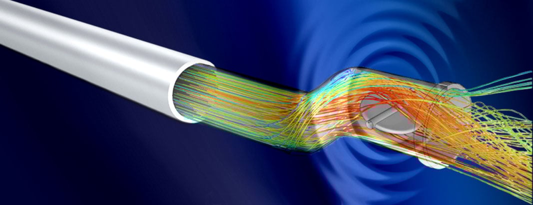
In this article, we provide an overview of the capabilities implemented in Ansys Fluent for addressing aeroacoustic challenges. The focus here is on the localization of sound sources — essentially answering the question: “Where is the noise coming from?” To explore this, we examine a pipe with a throttle valve and an outlet into the surrounding environment (see figure below). We assume broadband noise and aim to localize the sound sources, for example, to make geometric modifications or avoid certain operating conditions. This is particularly relevant for ventilation systems in buildings, where generated noise can be disturbing and undesirable.
Pipe with Throttle Valve | © CADFEM Germany GmbH
Sound generation & sound propagation in Ansys Fluent
Sound generation primarily occurs due to pressure fluctuations in turbulent regions, which is why we need to resolve these very finely in both time and space. Since sound waves can only propagate in compressible media, we must perform compressible simulations and discretize the relevant wavelengths with sufficient resolution. The time step must be chosen so that the information transported at the speed of sound moves no more than one cell per time step. For a fully resolved aeroacoustic analysis (CAA), this means that the transient, compressible Navier-Stokes equations must be solved with sufficient spatial and temporal resolution for a duration long enough to capture even the longest period of the sound waves.
Due to the high demands on mesh resolution and time step, a full CAA (Computational Aeroacoustics) simulation is very resource-intensive and often not feasible in practical applications. This is where acoustic analogy models come into play, in which sound propagation is computed using a separate wave equation solver. As a result, the flow field only needs to resolve the sound sources (turbulence), but not the sound waves themselves, allowing the fluid to often be treated as incompressible. Representatives of this model family include the Acoustic Wave Solver (AWS) and the Ffowcs Williams & Hawkings (FW-H) method. The latter is particularly used when large distances between the sound source and the receiver must be covered.
For the sole purpose of localizing sound sources, the previously described methods (CAA, FW-H, and AWS) are too computationally intensive. Therefore, Ansys Fluent also includes the simplest model group: the so-called broadband noise models. These are based on the solution of the steady Reynolds-Averaged Navier-Stokes (RANS) equations. Naturally, a steady CFD solution cannot provide transient results such as a frequency spectrum or sound wave propagation, which are inherently time dependent. As such, these models are only suitable for analyzing the sources of broadband noise. Their advantage lies in their low computational cost and the fact that they are purely post-processing methods (see figure).
Left: Ansys Fluent GUI & Acoustics. Right: Overview of Available Models in Ansys Fluent | © CADFEM Germany GmbH
Localizing Sound Sources in the Component
In our example – the pipe with the throttle valve – we want to get to the bottom of the noise. The goal is to understand where the sound originates, and which component contributes most significantly to noise generation. At this stage, we do not need any information about the actual sound pressure level at the receiver or the frequency spectrum—we are solely interested in the sound sources. Therefore, using the broadband noise models is sufficient for addressing this task. But which of the models shown in the figure above is the right one, and what are the differences between them?
Ansys Fluent offers four broadband noise models: Acoustic Power, Surface Acoustic Power, Lilley’s, and LEE Noise Source. The latter two require synthetic turbulence but offer no practical advantages, so they will not be considered further. To understand the difference between Acoustic Power and Surface Acoustic Power, we need to look at the classification of sound sources (see figure). The turbulent eddies in free jet turbulence behave acoustically like quadrupole sources (model: Acoustic Power), while wall-turbulence interactions behave like dipole sources (model: Surface Acoustic Power). Typically, quadrupole sources only become dominant at high Mach numbers.
In our case, we are dealing with a wall-bounded flow in a low Mach number regime. Therefore, it is expected that dipole sources dominate, making the Surface Acoustic Power model the appropriate choice. Once the broadband noise models are enabled in the Ansys Fluent GUI under Physics › Acoustics, they can be used for postprocessing. As shown in the figure below, the leading edge (LE) of the valve is clearly the primary source of noise. However, the underside of the trailing edge (TE) and the shaft itself also contribute to the generation of sound. For an A-B comparison, we can evaluate the total acoustic power under Results › Reports › Surface Integrals, which in this case is 8e-9 W.
Dipole & Quadrupole Sources, Right: Sound Source Analysis Using the Surface Acoustic Power Model. | © CADFEM Germany GmbH
Ansys Fluent GPU Performance Testing – Use Case
Ob im Maschinenbau, in der Luftfahrt oder bei der Produktentwicklung: Strömungssimulationen sind für präzise und schnelle Entwicklungsprozesse unerlässlich. Doch wie unterscheiden sich CPU- und GPU-basierte Simulationen, und was sind die wichtigsten Kriterien bei der Hardwarebewertung? Dieser Beitrag beleuchtet grundlegende Unterschiede, Leistungsmetriken und die Anwendungsmöglichkeiten von GPU- und CPU-Setups für Ihre CFD-Projekte.t

How to choose the right Aeroacoustic Model
In summary, we can say that in aeroacoustics, both the type of flow and the specific question being addressed are crucial. For external flows with a distant observer and questions about perceived loudness, we need a scale-resolved CFD simulation to accurately capture the turbulence (i.e., the sound sources), along with the FW-H model to bridge the distance between the observer and the sound source. If we are only interested in identifying the origin of the sound and the frequency spectrum is not of concern, the broadband noise models are worth considering – just as in our example. The table below provides possible simulation approaches for various scenarios and questions.
Why not examine your design for potential sound sources next time? All you need is a RANS analysis. If you're interested in the frequency spectrum at the receiver location, our aeroacoustics training course offers best-practice guidelines and the relevant expertise: Aeroakustik-Simulation: Schallentstehung in Strömungen | Seminar. Also, take a look at the Ansys Fluent GPU Solver – it's a real game changer in the realm of scale-resolved CFD when it comes to computation time. You can find more details in this TechArticle: Ansys Fluent GPU Performance Testing – Use Case.
Application Scenario |
Acoustic Question |
CFD Approach |
|
|
|
CFD |
Acoustics |
|
|
|
|
Automotive HVAC system |
Noise at driver and passenger sides |
SBES |
AWS oder CAA |
Wind in residential area |
Noise in traffic-calmed zones |
SAS or SBES |
AWS |
Headphone design |
Flow separation inducing sound |
WMLES |
CAA |
HVAC system in buildings |
Noise reduction / optimization |
RANS |
Broadband noise models |
Car side mirror |
Noise reduction / optimization |
RANS |
Broadband noise models |

Training Tip
Aeroacoustic Simulation – Sound Generated by Flowing Fluids
In this training course you will learn, how to tackle such problems generated by flow through or around components, vehicles, parts or systems with the help of numerical simulation and ANSYS Fluent.


Technical Editorial
Dr.-Ing. Marold Moosrainer
Head of Professional Development
+49 (0)8092 7005-45
mmoosrainer@cadfem.de