Welding Process Simulation Made Easy!
Sebastian Hoffmann
18.09.2026
TechArticle 26/08 | Weld Process Add-On: Toolbox for Weld Simulation
How do you get the perfect welding process right from the start? Welding process simulation helps master these complex manufacturing operations. Ansys supports the setup of the joining process with the new Weld Process add-on: weld direction and sequence can be varied with ease. This clears the way for calculating temperature field, weld distortion, and residual stresses.
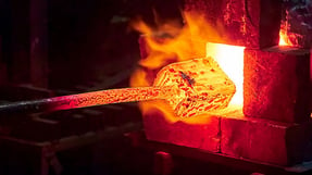
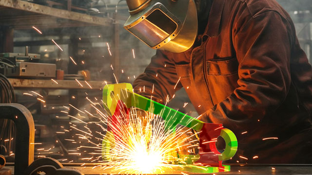
From the real welding process to digital simulation © CADFEM / Adobe Stock. Image AI-generated.
Summary
- Why is welding process simulation so complex? A moving heat source, Ekill/Ealive functionality, and the coupling of temperature field and structural mechanics: all of this is needed to capture these processes.
- How does the Weld Process add-on help? The new add-on is a practical toolbox that helps define the welding process as well as the direction and sequence of the weld seams.
- How flexibly can the welding process be adapted? Once the process is set up, different welding processes, parameters, and sequences can easily be realized.
Welding Process Simulation
Welding processes are complex procedures. They are characterized by a large amount of heat being introduced locally into a component. This locally melts the material, and the fusion of the material joins the components together. Welded assemblies typically consist of a large number of seams. Distortion is unavoidable. There is a wide variety of welding methods with many different process parameters. These have to be adapted depending on the application and component. How do you get this under control? It would help if the user were supported when setting up the process.
But the simulation is not simple either. First of all, this involves transient processes. We have to consider both thermal and structural mechanical effects. To capture the process, we need a moving heat source. Material is heated, melts, and then solidifies again. The weld seam forms step by step. To calculate the distortion, the time-varying temperature field must first be determined. And what happens if the welding sequence changes? Then the heat source suddenly moves along new paths, and we may have to adapt our model considerably.
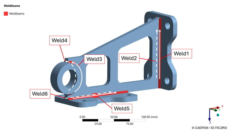
We want to approach these questions using an example. It is a welded assembly made up of several sheet metal parts joined by fillet welds. The assembly is joined in several locations and in different welding directions. Three-dimensional effects also play a role here: alongside seams in the X and Z directions, one seam runs tangentially along a round part that is welded into a round recess.

Geometry with weld seams and their corresponding directions. | © CADFEM / ID: 75C2RO

Weld Process Add-On
In order to depict the welding process, simplifications have to be made. Until now, solutions such as ACT extensions or APDL scripts were available for this. The new Weld Process add-on — a native Mechanical extension — combines much of this functionality and makes it easier to create weld models directly in the Mechanical application. Whereas in the past it could take hours to set up a model, this is now possible much faster with good preparation. The basic goal is to determine the temperature distribution during the process and to predict distortion and residual stresses.
Code:
# import libraries
import os
from ansys.geometry.core import launch_modeler_with_discovery
# create string with discovery code
cmd = """
# fix Small Faces with a smaller width of 1.5 mm
FixSmallFaces.FindAndFix(FixSmallFacesOptions(Width=MM(1.5)))
# define variables
bending_face = None
z_bending_face = float('inf')
# loop through faces
for face in GetRootPart().Bodies[0].Faces:
# get z coordinates and shape
z_cordinates = face.EvalMid().Point.Z
shape = face.Shape.Geometry.ToString()
# get bending face on the bottom
if (shape.Contains("Cylinder")):
if(z_cordinates < z_bending_face):
z_bending_face = z_cordinates
bending_face = face
# […] identify other important faces (clamping faces for example)
# save the faces in named selections
Selection.Create(bending_face).CreateAGroup("bending_face")
# […] also save other faces in named selections
"""
# create a text file and input the discovery code
fd = os.getcwd()
path = os.path.join(fd, "discovery.py")
with open(path, "w", encoding="utf-8") as file:
file.write(cmd)
# start discovery, open the geometry and run the code
modeler = launch_modeler_with_discovery(product_version = 251, hidden = True)
design = modeler.open_file(os.path.join(fd,"geometry.step"))
modeler.run_discovery_script_file(os.path.join(fd,"discovery.py"))
# save the finished geometry and delete the code file
design.save(os.path.join(fd,"geometry_prepared.scdocx"))
modeler.close()
os.remove("discovery.py")
Code:
# import libraries
import os
import ansys.meshing.prime as prime
from ansys.meshing.prime.graphics.plotter import PrimePlotter
# start client and assign lucid meshing
prime_client = prime.launch_prime()
model = prime_client.model
mesh_util = prime.lucid.Mesh(model=model)
# define path to geometry
fd = os.getcwd()
input_file = os.path.join(fd," geometry_prepared.dsco ")
# create a surface mesh
mesh_util.read(file_name=input_file)
mesh_util.surface_mesh(min_size=2.0)
# create a volume mesh and display
mesh_util.volume_mesh()
display = PrimePlotter()
display.plot(model, update=True)
display.show()
# save mesh
mesh_file_cdb = os.path.join(fd, "mesh.cdb")
mesh_util.write(mesh_file_cdb)

Weld Process Add-on. | © CADFEM / ID: KWF5KD
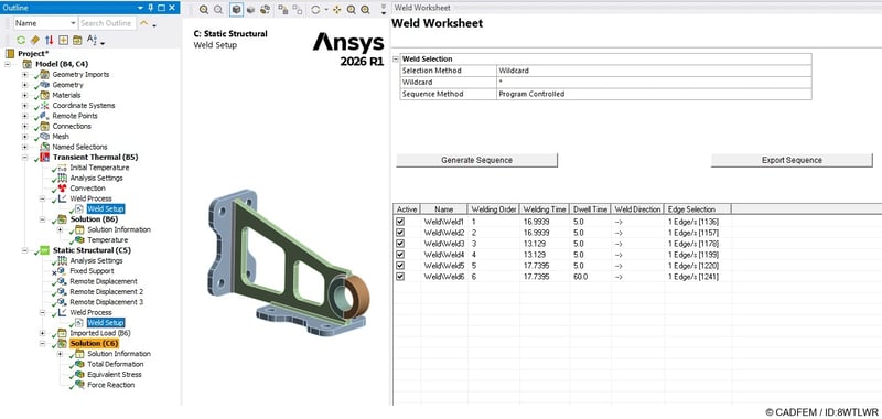
There are three calculation variants:
-
If you are only interested in the temperature distribution, a transient thermal analysis is sufficient — this is significantly less demanding and therefore a good first analysis.
-
There is also the option of running only a structural mechanical analysis. Since information on the temperature distribution is then missing, the thermal strains have to be calibrated using measurement data and scaled accordingly via the „Thermal Strain Scaling Factor."
-
The classic case is a transient thermal analysis followed by a sequentially coupled mechanical analysis
The weld seams are integrated as solid bodies, ideally named and numbered unambiguously.

Weld Setup | © CADFEM / ID: 8WTLWR
The order and direction of the seams can be defined, as can the pause times between individual seams. In addition, process parameters such as melting temperature, ambient temperature, and welding speed can be entered. It is precisely these parameters that largely determine how much the component distorts in the end. The elements in the weld seam are „clustered," meaning groups of elements are created. These clusters are activated one after another and supplied with heat, so that the weld seams build up step by step and a moving heat source is created. The user determines the size of the clusters. Optionally, a Goldak heat source can also be used.
Coupled Thermal and Mechanical Simulation
Since we are dealing with temperatures up to the melting temperature, the process simulation requires temperature-dependent material data. In addition, a plastic material model with likewise temperature-dependent stress-strain curves is required. Corresponding data can be found, for example, in the Engineering Data Sources under Additive Manufacturing Materials or in the Granta database. In our case of coupled simulation, the two analyses are solved sequentially, one after the other: first the temperature field, then the structural mechanics. The number of load steps results from the number of element clusters and any cooling steps.

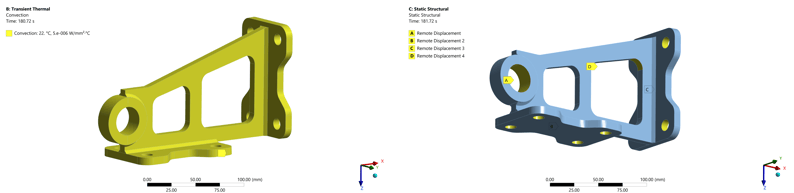
Convection boundary condition, thermal analysis (left), fixation points, structural analysis (right). | © CADFEM / ID: DPYW0C
Depending on the welding process, you can choose between two variants: for material deposition, element kill/alive technology is used to create the weld elements, e.g. in a fillet weld. To simulate the welding process without filler material, direct energy deposition simply applies heat, with no activation or deactivation of elements. The heat input itself can be defined via the applied temperature or the applied power. In the background, the reference temperature for the weld seam solid bodies is automatically set to the melting temperature.
Since we are modeling the entire process, we naturally also have to account for corresponding computation times. As so often, the challenge is to find the middle ground between a fast and a meaningful simulation. For a first attempt (at least for the weld distortion), a fairly coarse weld seam mesh with only a few elements in the weld seam cross-section can already give a good impression of the structure's behavior. Once our model is set up, we can very easily make changes to the weld sequence, the weld direction, or the process parameters.
How Hot Does It Get? The Heat Source over Time

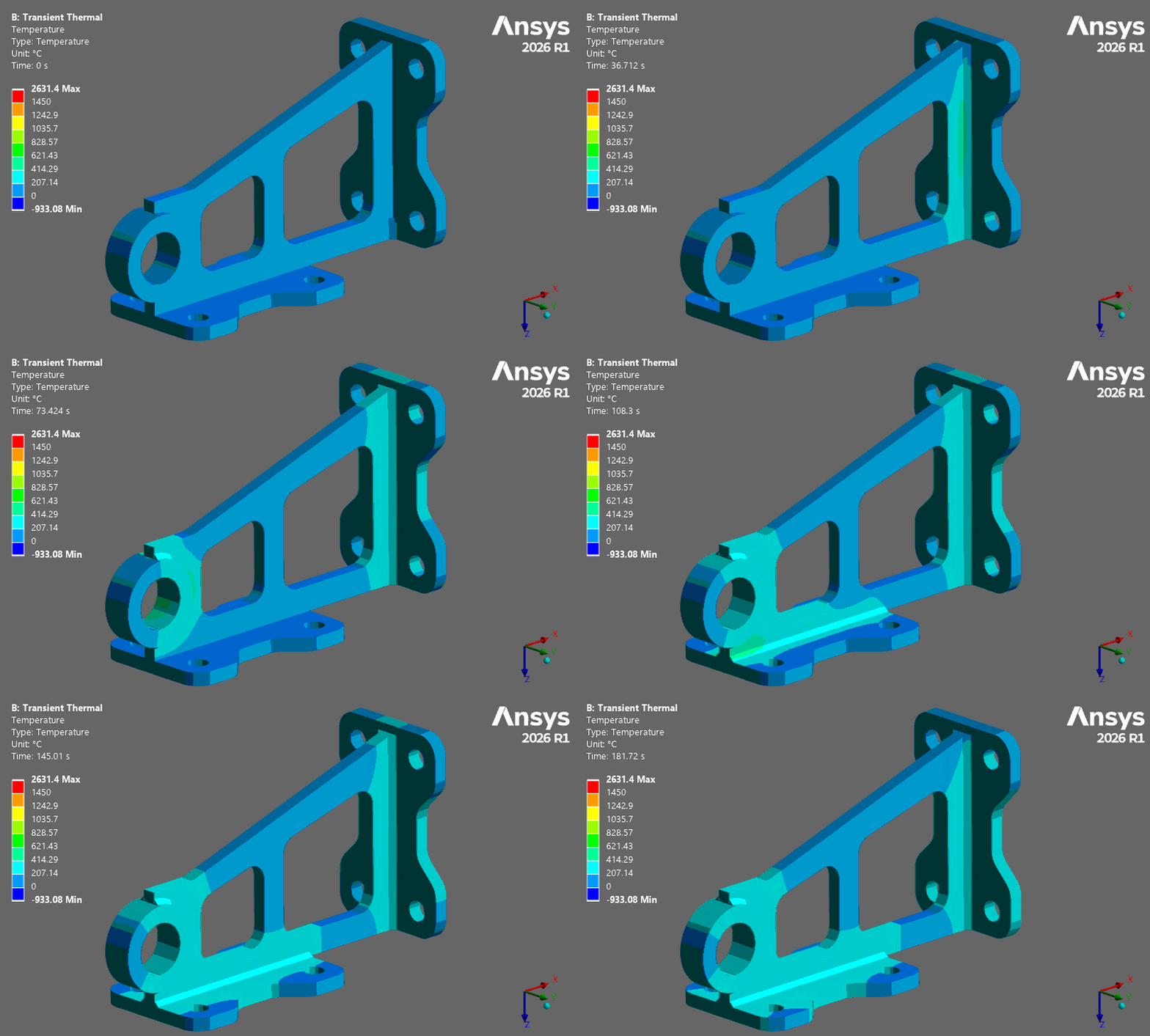
Temperature result at different points in time during the welding of a weld seam. | © CADFEM / ID: AG33J0
Probably the most exciting result of the transient thermal analysis is the changing temperature field during the process. Depending on how far the heat source has already progressed along the seam, every point in the component reaches its maximum temperature at a different time. A „special" result available only for the thermal part of the welding process simulation is the weld penetration result. It shows where and how strongly the heat penetrates the component, helping to identify critical areas (heat-affected zone). It is precisely there that the material's microstructure often changes due to the high thermal load, which can affect the later strength.
When you watch the temperature result animated, you can nicely observe the moving heat source. It is easy to see that at the start of the process, no weld seams are present yet — the seams form step by step, or „cluster by cluster," exactly as described earlier. This makes it possible to directly follow how element activation works in practice and how the heat actually spreads through the component in the process. This exact time-dependent development provides the basis for everything that is subsequently calculated in terms of distortion and residual stresses.
By the way, once the mechanical analysis is complete, you can also display the temperature result as a User Defined Result (expression: BFE). This has the advantage that you can additionally see the deformations. It is best to increase the displacement scale factor for this. At the same time, the temperature is shown as a contour plot. In the region of the heat source, you can nicely see the thermal strains this way.
TechArticle: Want more Young's Modulus?
Have you ever wanted to design a material according to your own ideas? A higher Young's modulus would be nice, wouldn't it? The way to achieve this is through the microstructure of the material. In this article, we look at how you can use Ansys Material Designer to determine the glass particle fraction that will allow you to double the Young's modulus of a plastic.
Code:
# import libraries
import os
from ansys.dpf import core as dpf
# open result file
fd = os.getcwd()
model = dpf.Model(os.path.join(fd,"result.rst"))
# get results and mesh
results = model.results
mesh = model.metadata.meshed_region
# extract displacement results
displacements = results.displacement()
field = displacements.outputs.fields_container()
# export the displacement field
my_export = dpf.operators.serialization.vtk_export()
my_export.inputs.file_path.connect(os.path.join(fd,"displacement.vtk"))
my_export.inputs.fields1.connect(field)
my_export.inputs.mesh.connect(mesh)
my_export.run()
# shutdown all dpf servers
dpf.server.shutdown_all_session_servers()
How Distorted Does It Get Now? Getting Bent Out of Shape?

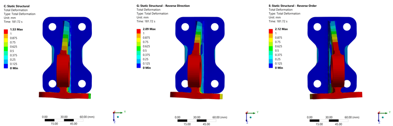
Total distortion after releasing all fixed supports except those on the rear plate, for different variants: initial welding sequence (left), initial welding sequence with reversed welding direction (center), reversed welding sequence (right); exaggerated deformation scale. | © CADFEM / ID: OVNNO4
If you reverse the sequence or direction of the weld seams — which is easy to change — the weld distortion changes significantly. For the variant with a changed welding direction, the distortion increases by almost 37% compared to the initial variant; for the variant with reversed welding sequence, by 39%. In this case, the structure deforms in the opposite direction (positive y-direction), while the other two variants deform in the negative y-direction.
The initial sequence turns out to be the one with the least distortion. With a sufficiently fine mesh, the residual welding stresses that develop after cooling to room temperature can also be evaluated.
Who really knows which sequence or welding direction is best? And who, please, wants to try them all out? For smaller assemblies like this one, you might still be able to estimate the tendency to distort, but for larger structures? That takes a lot of experience. How many possible combinations are there? The nice thing is: you basically no longer need APDL, but you can still intervene via APDL if needed.
And What Can I Take Away?
The example shows how a welding process can be set up and the process simulation carried out. The user is supported in this by the new Weld Process add-on. Among other things, it helps create variations of the welding sequence and direction as well as the process parameters.

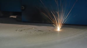
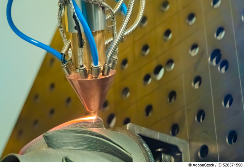
Additive manufacturing: laser metal deposition welding for repairing metal components. | © Adobe Stock / ID: 526371590

If you would like to learn for yourself how to carry out such temperature field analyses, take a look at our seminar „Simulation of Temperature Fields in Ansys Mechanical." A similar solution is also available for additively manufactured components: you can find out more in the seminar „Simulating Additive Manufacturing Processes in Metal Printing." We would also be happy to address your individual question on welding process simulation as part of a joint consulting project.
So don't shy away from welding process simulation! With the Weld Process add-on, you'll get into some serious welding — without breaking a sweat.
Ansys Fluent GPU Performance Testing – Use Case
Ob im Maschinenbau, in der Luftfahrt oder bei der Produktentwicklung: Strömungssimulationen sind für präzise und schnelle Entwicklungsprozesse unerlässlich. Doch wie unterscheiden sich CPU- und GPU-basierte Simulationen, und was sind die wichtigsten Kriterien bei der Hardwarebewertung? Dieser Beitrag beleuchtet grundlegende Unterschiede, Leistungsmetriken und die Anwendungsmöglichkeiten von GPU- und CPU-Setups für Ihre CFD-Projekte.t
More on the Topic
-
Simulation of Temperature Fields in Ansys Mechanical
Learn how to perform thermal analyses in Ansys Mechanical: best practice for heating and cooling tasks and determination of thermal stresses. This training is offered as a 3-day course or alternatively as a self-paced eLearning course.
-
Let's Simulate – Temperature Field with Feed
Welding without welding beads - Dr.-Ing. Jörg Neumeyer and Dr. rer. nat Sigrid Lang use simulation examples to discuss how heat and mass transport in solids and fluids can be represented. In this series, you will see the application of useful equations and the correct approach to how stationary temperature field calculations are done. Afterwards, you will be able to apply these helpful tips to effectively simulate temperature fields caused by welding processes. This is what makes this series a must for all engineers who want to deepen their knowledge of temperature measurement and simulation.
-
Simulating Additive Manufacturing Processes in Metal Printing
In this training, you will learn to use Ansys Mechanical to simulate the 3D printing process for components in order to optimize geometry, component orientation and warpage. This training is offered as a 1-day course.