EMFC Scale: How Simulation Makes Temperature Drift Visible

How does the EMFC scale really work?

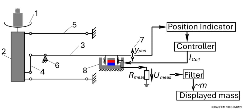
For scales used in pharmaceutical packaging lines, one thing is non-negotiable: precision (for the measurement engineers in the room: high resolution and high reproducibility). And speed. That leaves only one weighing principle: the EMFC scale, or electromagnetically force-compensated scale. When a mass is placed on the weighing pan (gently set down or dropped), it lowers along with the pan support. This motion transfers to the scale lever. A position indicator detects the deflection, and the controller drives a current through the copper coil in the field of the permanent magnet. The resulting Lorentz force counteracts the deflection until the lever is at rest again and the weight force is compensated.

Schematic representation of an EMFC scale. 1 – Weighing pan, 2 – Pan support, 3 – Scale lever, 4 – Coupling band, 5 – Parallel guide, 6 – Lever bearing with monolithic flexure joint, 7 – Position indicator, 8 – Electromagnetic actuator | © CADFEM / ID: KXNRMV

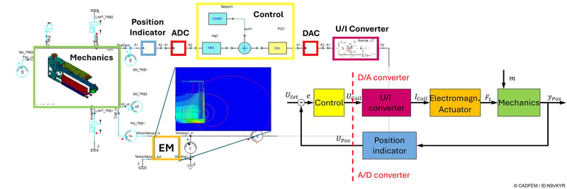
So much for the basic principle - but the question remains: how exactly does the controller determine the required compensation current? The coil current is linked to the mass being measured via a calibration factor. In practice, then, the scale does not measure a displacement but a current - captured via a reference resistor in series with the coil and converted into a mass using the calibration constant. That sounds straightforward. The real challenge, however, is that the mechanics, actuator and voltage-to-current converter influence each other - across the boundaries of physical domains. Every movement of the lever induces a back-voltage in the coil, which in turn feeds back into the converter.

In short: mechanics, electromagnetics and electronics constantly influence one another. This is exactly where a conservative modeling approach helps: instead of manually wiring these interactions as feedback loops, an energy-conserving formulation is used - familiar from SPICE simulations in electronics, but transferable to any physics domain. The feedback effects arise automatically, making the approach more robust - and considerably less error-prone. For the system simulation, the task now is to derive component models that are accurate yet fast to compute. The main components, mechanics and actuator, already exist as component models - reducing them and reusing this know-how is the obvious next step.

How Is the Mechanics Reduced to a Simulation-Ready Model?

The job of the scale mechanics is to relate the forces acting via mass and actuator to one another, without contributing anything to the equation itself — which is why the mechanism is friction-free and built with flexible monolithic flexure joints. A high lever ratio produces a large deflection for small mass changes, which contributes to the required high resolution. Use in packaging lines demands very fast settling, a property that is achieved particularly well with short, stiff levers — which creates a design conflict that is hard to resolve. The system simulation reliably evaluates this trade-off, provided the model correctly captures both statics and dynamics.

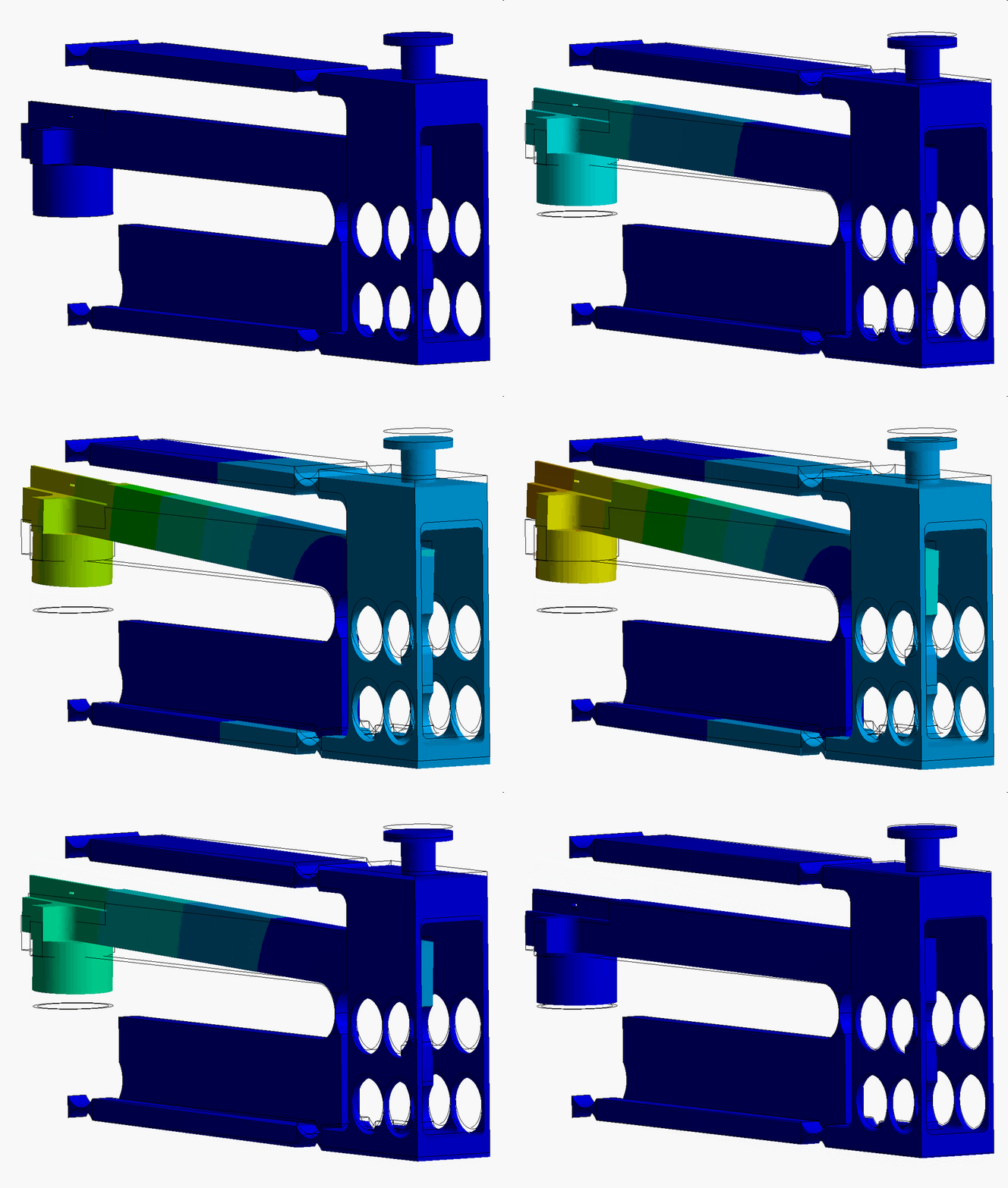
First mode shape of the scale mechanics. | © CADFEM / ID: VFZ3RT

Running a modal analysis reveals the following characteristics: the actually desired motion of the scale is represented by the first mode shape, while higher natural frequencies and their corresponding mode shapes produce bending and torsion modes that lead to unwanted vibrations. These natural modes have the convenient property of being orthogonal to one another. Or put more simply: any motion or (linear) deformation can be represented as a weighted superposition of the mode shapes. Truncating this basis shrinks the model considerably and also makes it very sparse, and therefore nicely fast to solve.

Exactly how this projection is found would go beyond the scope of this article. More details on modal reduction with SPMWRITE can be found here: Reduce components for system simulation. The reduced model thus quickly and accurately delivers everything we need: the static deflection and the dynamic behavior, including all the unwelcome higher-order modes. What we cannot account for is nonlinear behavior such as very large deflections - but the controller nips that in the bud anyway.

How Does Electromagnetics Enter the System Model?

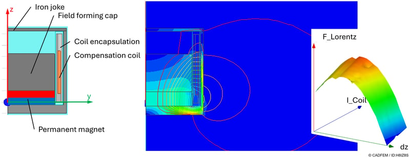
Design of the electromagnetic actuator (left), distribution of magnetic flux density B and field lines (center), Lorentz force as a function of coil current and coil position (right). | © CADFEM / ID: H8IZ8S

The resulting Lorentz force depends on the geometric configuration of the permanent magnet, pole plate and iron return path, as well as on material parameters, the number of coil turns and the coil diameter, the present coil current and the position of the coil in the air gap. The design goal is to keep all influencing parameters small during operation compared to the influence of the coil current, and to produce as linear a force-current characteristic as possible. The design found with Ansys Maxwell is integrated into the system simulation here by means of an ECE model (Equivalent Circuit Extraction).

ECE models represent a static condensation in the form of a lookup table: in a design of experiments, currents and positions are varied and the resulting forces and flux linkages are recorded along with them. The resulting model includes nonlinearities (for example due to saturation effects), but not transient effects such as eddy currents. Once created, ECE models deliver very good results in very short simulation times.

If the coil housing is made of a conductive material, the motion of the lever induces an eddy current in the housing. The resulting Lorentz force opposes the motion and represents significant damping. In this case, only a co-simulation would deliver correct results. If the housing, as assumed here, is made of non-conductive material or is slotted so that no eddy currents can form, the numerically far more favorable ECE model is preferable.

How Does an Overall System Emerge from Individual Models?

The system simulation still lacks a few further components for which typically no FE simulation exists that we could reduce. Even so, there is no need to forgo existing simulation know-how — for example, an existing SPICE model for the current source can be imported, or alternatively it can be represented in TwinBuilder using the components available there, as done here. For the controller and both the A/D and D/A converters, an FMU (functional mockup unit, see also fmi-standard.org) could likewise be imported from another tool, for example the control engineer's favorite tool. 

System model of the scale. | © CADFEM / ID: N9VKYR

The causal nature of the FMU (signal in at the front, signal out at the back) fits very well into the simulation chain in this context, since controllers are causal in nature too. Once a suitable model has been found for every component, validated on its own, and then combined into a system simulation, the behavior of the overall system can be simulated very quickly. The modular structure makes it easy and fast to swap components. If the system simulation shows that a bending mode of the lever, combined with the electronics, causes the weighing system to tend toward oscillation, the mechanical component's model can easily be replaced with an adapted model using a stiffer lever. To be on the safe side, more voltage headroom can be built into the electronics. If this tendency to oscillate is only discovered once the components are largely fixed and a first prototype has been built, it falls to the control engineer to fix it.

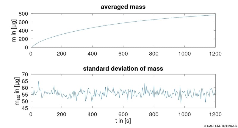
So much for the theory. But as mentioned at the outset, this elegant yet complex system has an unfortunate tendency to drift: the required stability of the mass determination of 100 µg is compromised.

Drifting mass signal: top, the mean value of the determined mass for the unloaded weighing pan; bottom, the corresponding standard deviation, both values each determined over 1 s after unloading the weighing pan. | © CADFEM / ID: H2RJ95

Why Does the Scale Drift?

The previous section explained the desired functioning of the scale, but environmental influences such as temperature, humidity or electromagnetic fields fell by the wayside. At this point, the complexity of the simulations should be kept manageable, so only temperature and its influence on system behavior are considered. The first question that arises is: where in the system is there a heat source? The largest share can be traced back to the actuator's power loss and quantified via the Joule heating of the coil. The electronics can be separated spatially from the scale mechanics fairly easily and therefore represent a heat source that is neglected here. tool, for example the control engineer's favorite tool.

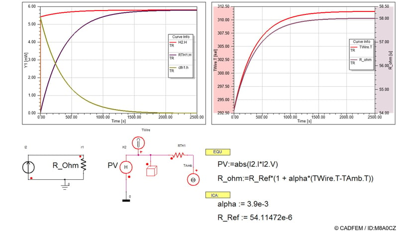
Modeling the self-heating of a coil. | © CADFEM / ID: M8A0CZ

With an isolated heat source, there is hope that only a single component might be affected by a changing temperature and would therefore be easy to control: the actuator's coil and its ohmic resistance. And indeed: the ohmic resistance does change when self-heating is added analytically. The clever colleague in electronics, however, had already thought of this and denies any blame: the analog-to-digital converter does not supply enough current to control the scale (otherwise a huge magnet would be needed, too expensive), so he built a voltage-controlled current regulator instead.

The scale controller thus sees a positional deviation of the lever, computes a correction signal, which the D/A converter turns into a voltage and passes on to the voltage-to-current converter. And that converter does what it is supposed to do, and regulates the current. Regardless of whether the coil's resistance drifts or not. According to the datasheet, the position indicator is also temperature-dependent and potentially the culprit. So the system simulation must be extended with two additional blocks: one that determines the temperature inside the scale housing, in particular at the position indicator, and a term for the temperature dependence in the description of the position indicator.

How Does MORiA Reduce the Temperature Field to the Essentials?

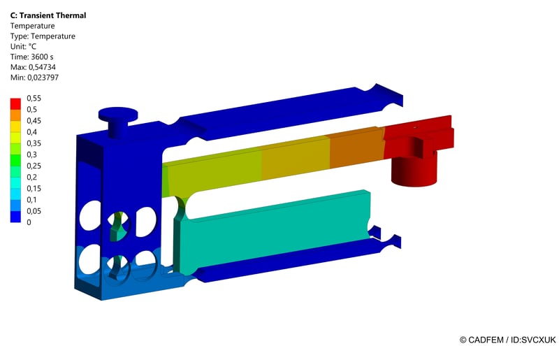
For the model order reduction of the thermal behavior, MORiA (Model Order Reduction inside Ansys) is used here. The principle of order reduction is similar here to the one described for structural mechanics: it involves projecting onto a subspace, which makes the model small, fast and easy to solve. Exactly how this projection is found would go beyond the scope of this article; the eLearning course on MORiA provides clarity on this.

Temperature field simulation of the scale. | © CADFEM / ID: SVCXUK

In short: we define our temperature field problem with all boundary conditions (convection at the scale surface, the coil's power loss as a unit load on the coil), and the system matrices are then written out automatically, the projection basis is found, and the model is reduced. The result is a state-space model (a compact mathematical model that links input and output quantities via a few internal state variables), which is fed with the coil power and quickly and accurately returns the temperature at the position indicator.

How Does the Simulation Make the Temperature Drift Visible?

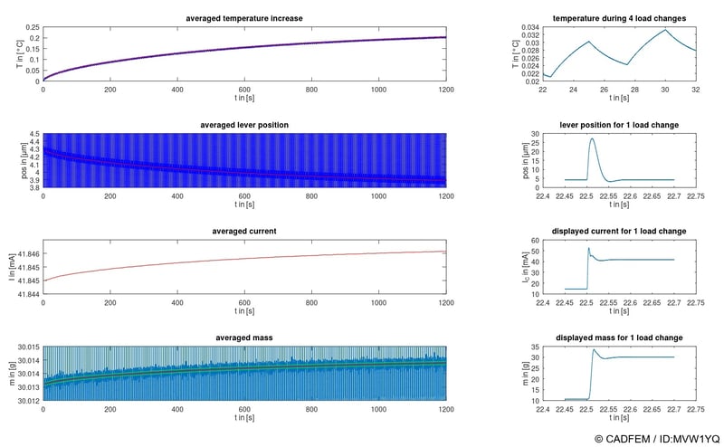
Once the system model has been extended with the reduced thermal model and fed with the power applied to the coil, a rise in temperature can be seen. Due to the temperature dependence now built in, the output signal of the position indicator changes. The controller keeps the lever's position constant by adjusting the signal for the voltage-to-current converter accordingly. We thus observe an inverse effect: as the position indicator drifts thermally, the real position of the scale lever is increasingly altered, and the stiffness of the monolithic flexure joints starts to play a role, which in turn changes the coil current and the displayed mass.

Results of the system simulation. | © CADFEM / ID: MVW1YQ

In short: we define our temperature field problem with all boundary conditions (convection at the scale surface, the coil's power loss as a unit load on the coil), and the system matrices are then written out automatically, the projection basis is found, and the model is reduced. The result is a state-space model (a compact mathematical model that links input and output quantities via a few internal state variables), which is fed with the coil power and quickly and accurately returns the temperature at the position indicator.